Direct and indirect observables

"They asked me for the temperature. What I actually held in my hand was a resistance, a wiring diagram, and a promise."

A Literal-Minded AI Agent

The measurand is rarely what the transducer touches

Ask a thermometer for the air temperature and it will answer without a single atom of it ever having sensed heat as heat: a bead of metal oxide inside merely grows more or less reluctant to pass current, and everything you read is inference laid on top of that reluctance. So begin where the honesty begins, by naming the quantity you were actually after: air temperature, blood oxygen, altitude, the speed of the car ahead. That target is the measurand. Now name the physical effect the sensing element actually produces at its terminals. For a thermistor it is electrical resistance; for a thermocouple it is a small voltage; for a pulse oximeter it is two light intensities; for radar it is a shift in the frequency of a returned wave. That terminal effect is the direct observable: the one quantity to which the transducer couples through a single, well-characterized physical step, and the only thing your electronics ever really digitizes.

Precisely, the measurand is the specific physical quantity a measurement is meant to determine, defined independently of any instrument: the true air temperature exists whether or not a thermistor is anywhere near it. It matters because it is the ground truth your whole pipeline is accountable to, the target you judge every later error against. You name and fix the measurand first, before choosing a sensor. You can reach the same measurand through very different direct observables (temperature from resistance, from a thermocouple voltage, or from infrared radiance), so stating it cleanly tells you which route you are actually committing to.

The gap between the two is the whole subject. A thermistor does not measure temperature; it is a resistor whose resistance happens to depend on temperature, and you read that dependence in reverse. This matters because the coupling, not your intention, sets what the raw number means. When the datasheet says a device measures temperature, it is compressing a longer and more honest sentence: this device produces a resistance, we have characterized how that resistance varies with temperature, and if you trust our characterization you may call the result a temperature. Keeping the direct observable in view is what lets you tell a broken instrument (its resistance genuinely changed) from a broken assumption (the resistance is fine, your conversion is wrong), a distinction we will return to throughout the chapter.

Indirection: computing what you wanted from what you got

Get this inversion wrong and a perfectly healthy sensor will lie to you with a straight face: aircraft have flown into terrain on altimeters that never twitched, and oximeters have reported comfortable oxygen over suffocating blood. The mechanism behind both is worth pinning down exactly. If the direct observable is the only thing the hardware ever truly hands you, then the quantity you actually wanted still has to be manufactured from it by computation. An indirect observable is any measurand you never touch directly and must reconstruct by applying a physical model to one or more direct observables. The reconstruction runs a known forward relationship backward. Resistance to temperature, pressure to altitude, round-trip photon time to distance, frequency shift to velocity: each is a small inverse problem, the same shape as the perception loop from Chapter 1, now made concrete for one sensor. Figure 2.1.1 lays out the chain that every indirect reading travels.

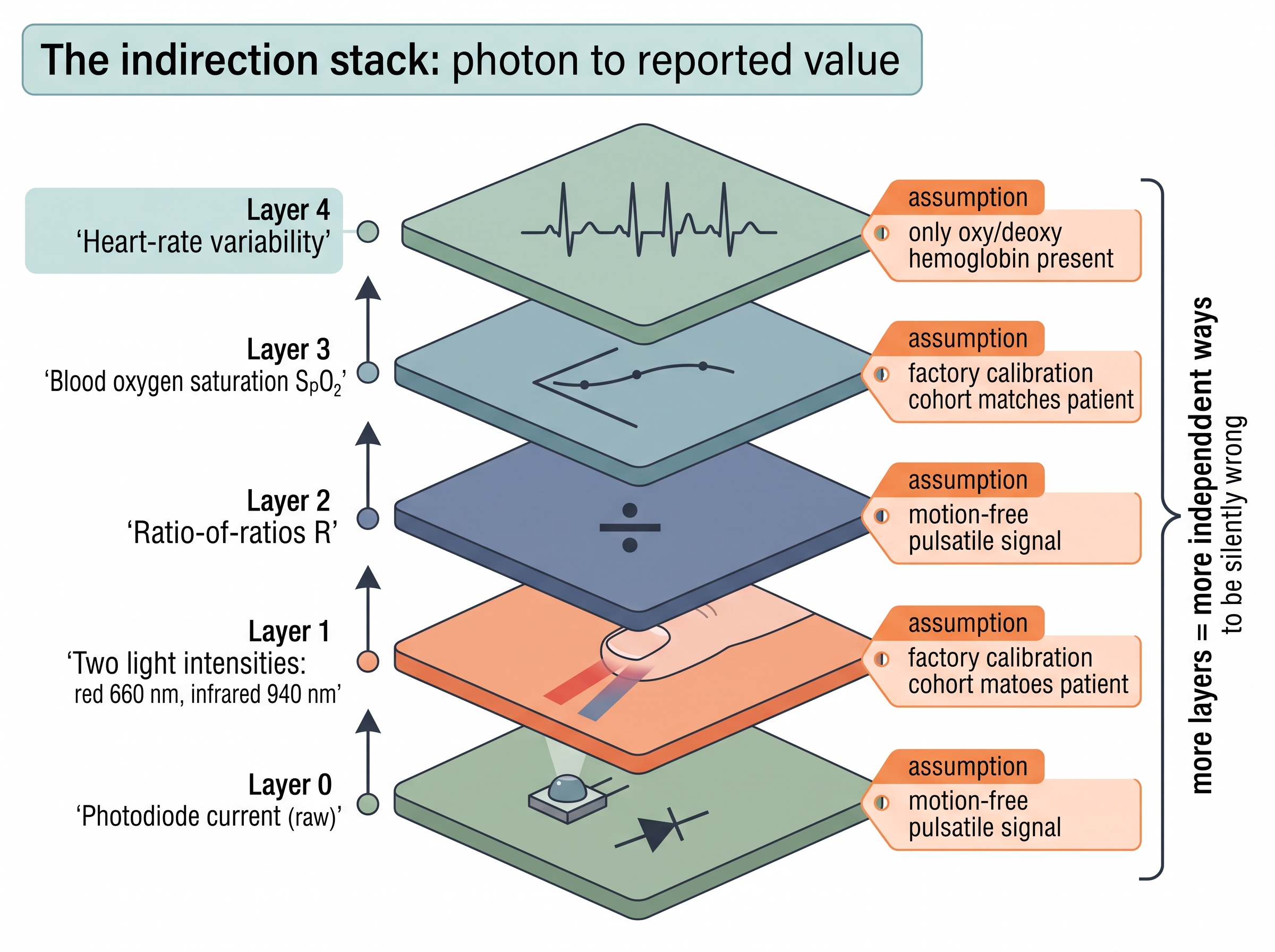
Indirection also stacks. A pulse oximeter recovers blood oxygen saturation from a ratio of two light absorptions, each itself inferred from a raw photodiode current. Heart-rate variability sits a level higher again, computed from beat intervals drawn from that same oxygen-modulated waveform. The number of layers between photon and reported value gauges how much modeling you are trusting, and how many ways the reading can be quietly wrong while the hardware runs perfectly. Radar makes the point in one clean step: the antenna sees only a frequency shift, and radial velocity falls straight out of the Doppler relation, where the frequency of a reflected wave shifts in proportion to the target's speed toward or away from the antenna, a technique Chapter 44 builds AI on top of. In short: name your observables truthfully and you will know where every future error is hiding before the first sample ever lands. Figure 2.1.2 illustrates stacked layers of indirection in a pulse oximeter (each layer adds an independent modeling assumption).

Every layer of indirection ships a hidden assumption

The model that turns a direct observable into an indirect one is valid only inside a domain, and that domain is a specification as real as any voltage range. A barometric altimeter recovers height from air pressure through the hydrostatic equation (the physical rule that the pressure at any height equals the weight of the air stacked above it), assuming a standard atmosphere. Let a weather front roll in and drop the sea-level pressure, and the altimeter reports a climb the aircraft never made; the pressure sensor is flawless and the altitude is fiction. A pulse oximeter's ratio-of-ratios calibration (the factory-fit curve that maps the red-to-infrared absorption ratio to a saturation value) assumes only oxygenated and deoxygenated hemoglobin are present; carbon monoxide poisoning violates that premise, and the device reads a reassuring high number over dangerously starved blood. A radar Doppler estimate assumes motion along the line of sight; a target crossing sideways registers almost no shift and is reported as nearly stationary.

None of these are noise, and no better or more expensive part cures them, exactly the trap Chapter 1 warned about. They are the conversion model applied where it does not hold. The practical discipline is simple. For every indirect observable in your pipeline, write down the assumptions its model rests on and the conditions that break them. Treat those conditions as failure modes to detect, not footnotes to ignore. When a learned model later consumes this signal, it inherits the validity domain whether or not anyone told it. A network trained only on sea-level flights has never seen the altimeter's front-passage lie and will trust it blindly, a leakage-of-context problem that returns in Chapter 4 when we reason about uncertainty formally.

Because the conversion is just arithmetic on a known relationship, it is also the kind of thing a library encodes once and reuses forever. Consider the workhorse example: turning a thermistor's resistance (direct) into temperature (indirect) through the Steinhart-Hart equation,

where \(T\) is absolute temperature in kelvin, \(R\) is the measured resistance, and \(A, B, C\) are coefficients from calibration. Listing 2.1 evaluates it directly so you can see the whole inversion in one place.

import numpy as np

def thermistor_temperature_c(resistance_ohms, A, B, C):
    """Steinhart-Hart: direct observable (resistance) -> indirect observable (temperature)."""
    lnR = np.log(resistance_ohms)
    inv_T = A + B * lnR + C * lnR**3       # 1 / T, with T in kelvin
    return 1.0 / inv_T - 273.15            # convert kelvin to Celsius

# Typical 10k NTC coefficients (from a calibration sheet):
A, B, C = 1.129e-3, 2.341e-4, 8.775e-8
for R in (32650, 10000, 3600):            # cold, nominal, warm
    print(f"{R:6d} ohm -> {thermistor_temperature_c(R, A, B, C):5.1f} C")

As Listing 2.1 shows, the physics of the inversion is a three-term polynomial in \(\ln R\); the risk lies almost entirely in the coefficients and their validity range, not in the arithmetic.

import board, adafruit_thermistor
t = adafruit_thermistor.Thermistor(board.A1, 10000, 10000, 25, 3950)
temperature_c = t.temperature      # resistance read, model inverted, range-checked

Why the distinction organizes the rest of this book

The GPS receiver sat at the deep end of this spectrum, and laying every sensor out along the same axis is exactly what makes the rest of the book fall into order. Sort any sensing task by how deep its measurand sits below the transducer and the book's structure appears. Shallow, nearly-direct observables (a thermocouple voltage, a raw accelerometer force) need clean acquisition and good calibration, the concerns of the rest of Chapter 2 and of Chapter 3. Deep, heavily-modeled observables (position from satellite timing, activity from motion, oxygenation from light) need estimation, fusion, and learned inversion, the concerns of Parts III onward. The design question for any new sensor is always the same two-parter: what is the direct observable I truly measure, and how many modeling assumptions stand between it and the number I report. Answer both plainly and you know where your errors will come from before you collect a single sample.

What's Next

In Section 2.2, we stop asking what a sensor observes and start asking how well: resolution, the smallest change it can distinguish; sensitivity, how strongly its output moves per unit of input; and dynamic range, the span from the faintest signal it can register to the loudest it can survive. Those three numbers decide whether the direct observable you just learned to name carries enough information to invert at all.