Resolution, sensitivity, dynamic range

"They asked me to detect a whisper and a thunderclap with the same ear, and to tell apart two whispers a hair's breadth apart. I asked which one mattered more, and they said yes."

An Overspecified AI Agent

Section 2.1 established the measurement model \(x = h(s) + \eta\): a hidden state \(s\) passes through the sensor response \(h(\cdot)\) and is digitized into a reading \(x\). This section characterizes the properties of that pipeline that cap its information content, deliberately setting aside the statistics of the noise term \(\eta\) (the subject of Section 2.3) and the failure of \(h(\cdot)\) at its extremes (Section 2.4). We assume only basic calculus and the notion of the transfer function from the previous section. If quantization and sampling feel unfamiliar, they are treated in depth in Chapter 3.

Resolution: the smallest distinguishable change

What. Resolution is the smallest increment of the measured quantity that produces a detectable, repeatable change at the output. Why it matters. It is a hard floor on discrimination. If two states differ by less than one resolution step, the sensor reports the same value for both. No filter, no network, and no amount of averaging over those identical readings can separate them. How it arises. Two mechanisms set it. The first is quantization. An analog-to-digital converter (ADC) with \(N\) bits carves its full-scale span \(V_\text{FS}\) (the total input range from the bottom to the top of its measuring window) into \(2^N\) levels, so the least significant bit (LSB) step, the smallest change it can represent, is

$$\Delta = \frac{V_\text{FS}}{2^{N}}.$$

A 12-bit converter spanning \(\pm 2\,\text{g}\) on an accelerometer resolves \(4\,\text{g} / 4096 \approx 0.98\,\text{mg}\) per step. The second mechanism is the analog noise floor. Even before digitization, thermal and electronic noise blur the output, so a converter with more bits than the analog stage warrants only digitizes that noise. The honest figure is the effective number of bits (ENOB), which discounts the nominal bit count by the measured noise. Resolution is also spatial and temporal, not only in amplitude: a thermal camera's resolution is its pixel pitch on the scene, and a heart-rate sensor's temporal resolution is set by its sampling interval. But the size of the smallest step the output can show says nothing about how far the output actually swings when the world nudges it, and that slope is the next thing to pin down. In short: what the front end throws away in one step, no downstream algorithm can ever get back.

Sensitivity: how hard the needle moves

What. Sensitivity is the slope of the transfer function: the change in output per unit change in the input, \(\;S = \mathrm{d}x / \mathrm{d}s\). For a linear sensor it is a single constant (a load cell might give \(2\,\text{mV/V}\) at full load; a photodiode's responsivity (its sensitivity, the output current produced per unit of incident optical power) might be \(0.6\,\text{A/W}\)). Why it matters. Sensitivity governs how a fixed amount of input maps onto the converter's steps, and so it interacts directly with resolution. A high-sensitivity sensor spreads a small physical change across many ADC codes, making that change easy to see. A low-sensitivity sensor compresses the same change into a fraction of one code, where it vanishes. How to reason about it. The catch is that sensitivity and range pull in opposite directions. Cranking gain to boost sensitivity moves faint signals up into many codes. But it also drives strong signals off the top of the scale into saturation (the ceiling where more input no longer moves the output). This is why sensitivity is a design knob, not a virtue to maximize blindly.

"Sensitive" and "high-resolution" are not the same claim, though they are linked. Sensitivity is a property of the analog transduction (slope); resolution belongs to the whole chain, including the converter (step size). Raising sensitivity lifts effective resolution only until you hit noise or saturation, where more gain buys nothing. What actually limits detection of faint signals is the ratio of sensitivity to noise, which is where Section 2.3 on signal-to-noise ratio takes over. Resolution and sensitivity each describe behavior near a single operating point; the remaining question is how wide a span of inputs the sensor can straddle before it clips at the top or vanishes into the floor at the bottom.

Dynamic range: from the faintest to the loudest

What. Dynamic range is the ratio of the largest signal a sensor can measure (its full scale, just below saturation) to the smallest it can resolve (its noise floor or one quantization step, whichever is larger). Because that ratio spans orders of magnitude, it is quoted in decibels, and for a converter it maps neatly onto bit depth:

The decibel (dB) is a logarithmic unit for the ratio of two amplitude or power quantities: for amplitudes, it is \(20\log_{10}\) of the ratio. It matters because sensor spans routinely cover many orders of magnitude, and a log scale compresses an unwieldy ratio like 1,000,000-to-1 into a readable 120 dB, while turning multiplicative gains into additive ones (every 20 dB is one factor of ten in amplitude, and 6 dB is roughly a factor of two, which is exactly why each extra converter bit adds about 6 dB). Reach for decibels whenever a ratio spans decades or you want to add stage gains by hand; keep plain linear units when the quantities are close together and an absolute difference, not a ratio, is what you care about.

$$\text{DR}_\text{dB} = 20 \log_{10}\!\left(\frac{x_\text{max}}{x_\text{min}}\right) \approx 6.02\,N + 1.76 \;\text{ for an ideal } N\text{-bit converter}.$$

Why the span decides the deployment

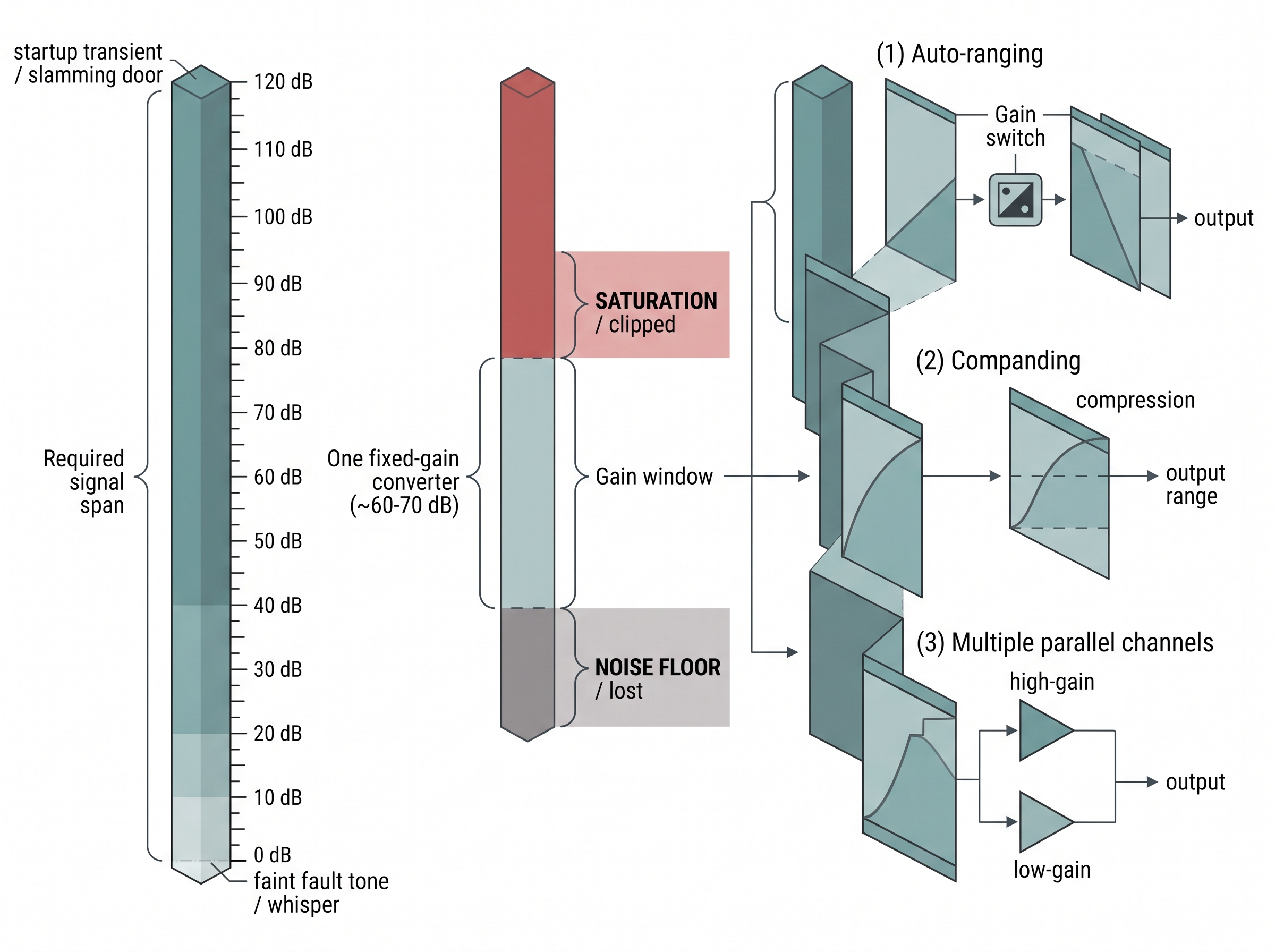
Why it matters. The physical world routinely presents signals across a huge range within one deployment. A microphone in a car must handle a quiet cabin and a slamming door; an automotive lidar return from a black tire at range and a retroreflective sign differ by many orders of magnitude; an inertial measurement unit (IMU) on a drone sees both gentle hover drift and the shock of a hard landing. If the required span exceeds the sensor's dynamic range, you are forced to choose which end to sacrifice, and something important gets clipped or lost in the noise. How to extend it. When one fixed setting cannot cover the span, systems use auto-ranging (switching gain on the fly, as a camera does with exposure), companding (compressing large signals nonlinearly), or multiple parallel channels. Each buys range at the cost of complexity, latency, or a discontinuity the downstream model must be told about. Note that the floor is set by noise (Section 2.3) and the ceiling by saturation (Section 2.4); dynamic range is the clean summary of the two you own from this section. Figure 2.2.1 illustrates Dynamic-range extension: covering a span wider than one converter can hold.

import numpy as np

def adc_specs(v_full_scale, n_bits, noise_rms):
    step = v_full_scale / (2 ** n_bits)          # quantization resolution (LSB)
    enob = n_bits - np.log2(max(noise_rms / step, 1.0))  # bits lost to noise
    dr_db = 20 * np.log10(v_full_scale / max(noise_rms, step))
    return step, enob, dr_db

for bits in (8, 12, 16):
    step, enob, dr = adc_specs(v_full_scale=4.0, n_bits=bits, noise_rms=3e-3)
    print(f"{bits:2d}-bit: step={step*1e3:7.3f} mV  ENOB={enob:4.1f}  DR={dr:5.1f} dB")

The snippet above makes the central trade concrete. Holding the analog noise fixed at 3 mV, the 8-bit and 12-bit converters gain real resolution, but the 16-bit part reports far more nominal precision than its ENOB, because the noise floor, not the bit count, sets the true smallest distinguishable step. This is why "how many bits" is usually the wrong first question; "what is the ratio of the loudest signal I must not clip to the faintest I must still see" is the right one.

All three specifications live on a single picture, the sensor's transfer curve. Figure 2.2.1 plots output against input and reads each specification straight off the geometry: sensitivity is the slope of the curve, resolution is the height of one quantization step along it, and dynamic range is the full vertical span from the noise floor at the bottom to the saturation ceiling at the top.

from scipy.signal import periodogram
f, pxx = periodogram(samples, fs=fs, window="blackmanharris")
# locate fundamental bin, sum the rest as noise+distortion, then:
# ENOB = (SINAD_dB - 1.76) / 6.02

Matching the three to the task

Pick a sensor's specifications for their datasheet glamour rather than the task, and you learn of the mismatch only after deployment: the fault tone you needed to hear sits buried under a single bit, or the startup transient you forgot to budget for clips on every power-up. The three specifications are not chosen in isolation; they are matched to what the application actually needs to distinguish, and against each other. Start from the decision the system must make, translate it into a required smallest distinguishable change (this sets resolution and, through the noise floor, the needed sensitivity) and a required span of operating conditions (this sets dynamic range). Only then pick hardware. A gesture classifier on an inertial sensor needs modest resolution but wide range to survive impacts; a tremor-monitoring clinical device needs the opposite, fine resolution over a narrow band. Getting this mapping right is upstream of every model you will train, and it feeds directly into how you reason about what the resulting estimates can and cannot claim, which is the uncertainty machinery of Chapter 4.

What's Next

Section 2.3 opens up the noise term \(\eta\) kept sealed here. Resolution and dynamic range both bottomed out on a "noise floor" we treated as a given; the next section names the physical sources of that floor (thermal, shot, flicker, quantization), shows how they combine, and turns the vague phrase "signal-to-noise ratio" into a quantity you can compute, budget, and improve.