Section 3.1: Sampling, aliasing, and the Nyquist limit

"They told me the wheels were spinning backwards. The wheels were fine. My eyes were just sampling too slowly, and no amount of model capacity fixes a frame that was never captured."
A Chastened AI Agent

Prerequisites

This section assumes you know that a sensor produces a continuous voltage that an analog-to-digital converter (ADC) turns into numbers, the measurement model $x = h(s) + \eta$ developed in Chapter 2, and the idea that a signal carries energy at various frequencies. Nothing more. The frequency-domain machinery used lightly here (the Fourier view of a signal) is built out in full in Chapter 7, and the filters that enforce the rule we derive are the subject of Chapter 6. A short trigonometric-identity refresher lives in Appendix A.

Why this section is the hinge of the chapter

Every digital sensor makes the same silent decision millions of times per second: it looks at the world, writes down a number, and then closes its eyes until the next tick. What happens between the ticks is gone forever. This section establishes the one law that governs whether the numbers you kept are enough to reconstruct what you missed, or whether they are a convincing lie. The Nyquist-Shannon sampling theorem is not a piece of trivia; it is the reason a 100 Hz accelerometer cannot see a 1 kHz bearing fault, the reason a cheap camera turns helicopter blades into a slow crawl, and the reason no downstream model, however large, can recover information that sampling threw away. Get the sample rate wrong at acquisition and the rest of the book cannot save you.

Hand a model twenty numbers and ask it which continuous world produced them: without a single guarantee about that world, it cannot say, and neither can you. We work with the notation from Chapter 1: the continuous signal at the transducer is $x(t)$, and sampling produces the discrete sequence $x[n] = x(nT_s)$, where $T_s$ is the sampling period and $f_s = 1/T_s$ is the sampling rate in samples per second (hertz). The whole section answers one question: given $x[n]$, what can we truthfully claim about $x(t)$?

The sampling rate $f_s$ is the number of measurements the converter records each second, and its reciprocal $T_s$ is the fixed gap between consecutive readings. It matters because it silently caps the fastest change the sensor can ever witness. The sampler discards everything the analog world does between two ticks, so $f_s$ is a hard ceiling on observable detail, not a software knob you can raise after the fact. Mechanically, a clock triggers the ADC once every interval $T_s$, freezing a single instantaneous value per tick. Reach for a high $f_s$ when the signal carries fast transients: impacts, sharp edges, high-pitched tones. Settle for a lower rate only when you can guarantee the content of interest is slow, and always pair it with an analog filter. Every extra sample per second costs power, bus bandwidth, and storage downstream.

Sampling: turning a function of time into a list of numbers

Get this one operation wrong and a $2,000 accelerometer becomes a random-number generator: the bearing fault it was bolted on to catch simply never appears in the data, no matter how sophisticated the model reading that data later is. Seeing why begins with what sampling does to a signal's frequencies. What sampling does is deceptively simple. It multiplies the continuous signal by an infinite train of impulses spaced $T_s$ apart and keeps only the values that land on the ticks. Why it is subtle is that this operation is not lossless in general, yet under a precise condition it loses nothing at all. How we know is the sampling theorem, and the fastest route to it runs through the frequency domain.

Multiplying a signal by an impulse train in the time domain convolves its spectrum (convolution being the sliding overlap-and-sum operation that stamps one shape at every position of another) with an impulse train in the frequency domain. This trade of multiplication for convolution whenever you cross between the time and frequency domains is a standard property of the Fourier transform; we take it on faith here and build it out in Chapter 7. The practical consequence is that sampling takes the original spectrum $X(f)$ and copies it, endlessly, centered at every integer multiple of $f_s$:

$$X_s(f) = f_s \sum_{k=-\infty}^{\infty} X(f - k f_s).$$

Picture the true spectrum as a single hump of content occupying frequencies up to some highest frequency $f_{\max}$. After sampling, that hump is stamped out at $0, \pm f_s, \pm 2f_s,$ and so on. If the copies do not touch, you can isolate the original with an ideal low-pass filter and recover $x(t)$ perfectly. If they overlap, the overlapping energy adds together and the original is unrecoverable. That overlap is aliasing, and avoiding it is the entire game. Figure 3.1 contrasts the two outcomes side by side: the top row shows spectral copies with clear gaps, the bottom row shows copies packed too tightly and colliding.

Figure 3.1. Sampling replicates a signal's spectrum at every integer multiple of $f_s$. Top: when $f_s > 2f_{\max}$ the copies leave a gap, so an ideal low-pass filter recovers the baseband exactly. Bottom: when $f_s \le 2f_{\max}$ the copies reach past the Nyquist frequency $f_s/2$ (half the sampling rate, defined formally in the next section) and collide (orange wedge), summing energy that no filter can separate afterward. That collision is aliasing.

The Nyquist limit: the one inequality to memorize

The copies of the spectrum stay clear of each other exactly when the sampling rate is more than twice the highest frequency present in the signal:

$$f_s > 2 f_{\max}.$$

The quantity $f_s/2$ is the Nyquist frequency: the highest frequency a given sample rate can represent without ambiguity. The threshold $2 f_{\max}$ is the Nyquist rate: the slowest you are allowed to sample a signal band-limited to $f_{\max}$, meaning it carries no energy at any frequency above $f_{\max}$. The Nyquist-Shannon sampling theorem states the payoff precisely: a signal containing no energy at or above $f_s/2$ is completely determined by its samples, and can be reconstructed exactly by sinc interpolation (summing shifted, scaled $\sin(\pi t)/(\pi t)$ kernels, one per sample). This is a remarkable claim. A continuous object with uncountably many values is pinned down, with zero error, by a countable list of numbers, provided it was band-limited first. In short: what the sampler never captured, no later stage can ever return.

Checkpoint

So far: the Nyquist frequency is half your sample rate ($f_s/2$), the Nyquist rate is twice the signal's highest frequency ($2f_{\max}$), and the sampling theorem says that whenever the first exceeds the second the samples pin the signal down exactly, sinc interpolation being the recipe that rebuilds it.

Common Misconception

The misconception is "sample at twice the highest frequency I care about." The theorem is about twice the highest frequency present at the converter, not the highest frequency you happen to find interesting. A 40 Hz signal of interest riding on top of unfiltered 3 kHz electrical hum still needs that hum removed before the ADC, or the hum folds down and corrupts your 40 Hz band; sampling faster than 80 Hz does nothing about energy you never filtered out. Nyquist constrains what is physically in the wire, not what is in your intentions.

The insight worth carrying to every deployment

Bandwidth, not sample rate, is the real budget. Doubling your sample rate is worthless if the signal already fits below the old Nyquist frequency, and it is insufficient if content lives above it. The design question is never "is 1 kHz fast enough?" in the abstract; it is "what is the highest frequency I care about, and have I guaranteed nothing lives above it before the converter fires?" That guarantee comes from a physical anti-alias filter in front of the ADC, not from software, because once aliasing has folded two frequencies onto the same sample, no algorithm can tell them apart again.

Aliasing: what a violated inequality actually looks like

When $f_s \le 2 f_{\max}$, a frequency $f$ above the Nyquist limit does not disappear. It folds back and masquerades as a lower frequency. The impostor frequency is

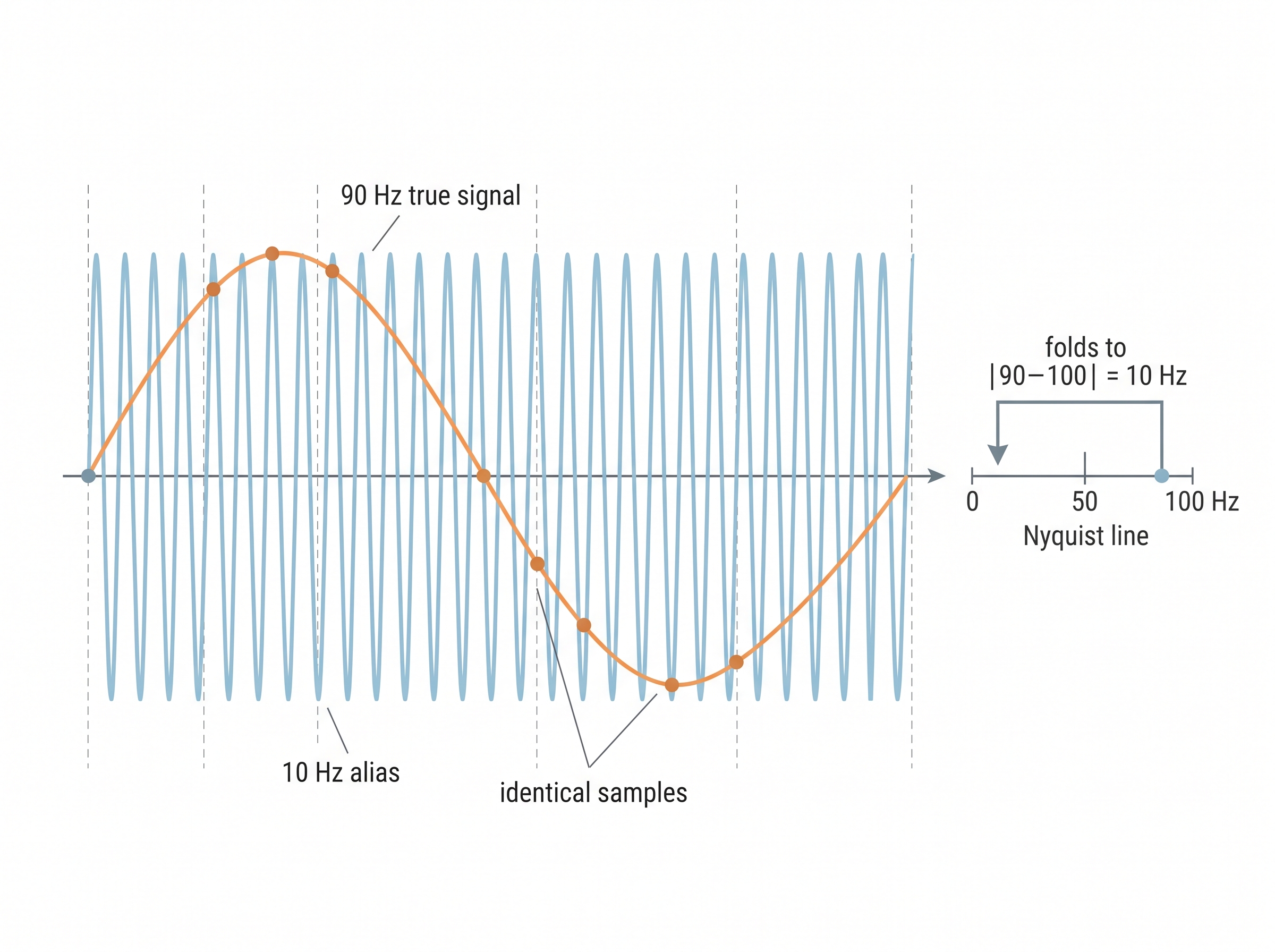
$$f_{\text{alias}} = \lvert f - k f_s \rvert,$$

where $k$ is the integer that lands the result in $[0, f_s/2]$. A 90 Hz vibration sampled at 100 Hz reappears as a $\lvert 90 - 100 \rvert = 10$ Hz vibration, indistinguishable from a real 10 Hz oscillation. Film's "wagon-wheel" effect is the same arithmetic: a wheel turning just under the frame rate seems to creep backward, each frame catching it short of a full turn. The code below samples a 90 Hz tone at 100 Hz and shows its samples matching a 10 Hz tone value for value.

Mental Model

Think of a 12-hour clock face. Ask it the time at 3 o'clock and again at 15:00, and the hand points to exactly the same spot: the dial has folded 15 back to 3 by quietly subtracting 12. It cannot tell you which of the two you meant, because the "24" of real time was wrapped into the "12" the face can display. Aliasing is that identical wrap. The sample grid can only display frequencies up to $f_s/2$, so a 90 Hz tone sampled at 100 Hz gets folded, $\lvert 90 - 100\rvert = 10$, and lands on the same "3 o'clock" as a true 10 Hz tone. Subtracting a multiple of $f_s$ is the clock subtracting a multiple of 12, and once the hand has moved, no glance at the dial can undo the wrap.

import numpy as np

fs = 100.0                      # sampling rate (Hz): Nyquist = 50 Hz
n = np.arange(20)               # 20 sample indices
t = n / fs                      # the sampling instants

true_signal = np.cos(2 * np.pi * 90 * t)    # 90 Hz: above Nyquist
alias        = np.cos(2 * np.pi * 10 * t)   # 10 Hz: the impostor

# The two continuous signals are completely different, yet on the grid...
print("max |difference| on the sample grid:",
      np.max(np.abs(true_signal - alias)))   # -> ~1e-14, i.e. identical

f_alias = abs(90 - round(90 / fs) * fs)
print(f"90 Hz sampled at {fs:.0f} Hz masquerades as {f_alias:.0f} Hz")

A 90 Hz cosine and a 10 Hz cosine, evaluated only at the 100 Hz sampling instants, produce byte-for-byte identical sample sequences. The difference on the grid is at floating-point noise level, which is the whole tragedy of aliasing: the samples cannot distinguish the honest signal from the impostor.

Run it and the printed difference is around $10^{-14}$. The two tones are physically distinct sounds, yet the sampler wrote down the same twenty numbers for both. This is why aliasing is dangerous rather than merely lossy: it does not blur the signal, it fabricates a plausible false one that looks like clean low-frequency data your model will trust. Figure 3.1.1 illustrates frequency folding (aliasing in the time domain).

Frequency folding (aliasing in the time domain) — Figure 3.1.1: A 90 Hz cosine and a 10 Hz cosine take identical values at every 100 Hz sampling instant, so the fast tone folds across the 50 Hz Nyquist line and masquerades as the slow one.

Step-Through: folding a frequency to its alias

Trace the fold formula $f_{\text{alias}} = \lvert f - k f_s \rvert$ with a real number, sampling a 130 Hz tone at $f_s = 100$ Hz (so the Nyquist frequency is 50 Hz). We want the integer $k$ that lands the result inside $[0, 50]$.

Try $k = 0$: $\lvert 130 - 0 \times 100 \rvert = 130$ Hz. That is above 50 Hz, so it is not the answer; keep folding.
Try $k = 1$: $\lvert 130 - 1 \times 100 \rvert = \lvert 30 \rvert = 30$ Hz. That sits inside $[0, 50]$. Done.
Sanity check $k = 2$: $\lvert 130 - 200 \rvert = 70$ Hz, back outside the band, confirming $k = 1$ was the right choice.

So a 130 Hz tone recorded at 100 Hz is written down as an indistinguishable 30 Hz tone. Verify it directly: at the sample instants $t = n/100$, $\cos(2\pi \cdot 130\, t)$ and $\cos(2\pi \cdot 30\, t)$ agree for $n = 0$ they are both 1, for $n = 1$ both $\cos(2.6\pi) = \cos(0.6\pi) \approx -0.309$, for $n = 2$ both $\cos(5.2\pi) = \cos(1.2\pi) \approx -0.809$. Same numbers, two different tones.

The bearing fault the monitor could not see

An industrial team instrumented a gearbox on a conveyor line with an accelerometer logging at 200 Hz, reasoning that the shaft turned at only 25 Hz so 200 Hz was "eight times faster than anything interesting." For months the vibration trace looked healthy. Then a bearing failed catastrophically. The post-mortem found the smoking gun: the failing bearing's characteristic defect frequency sat near 1.3 kHz, and its harmonics folded down through the 100 Hz Nyquist limit into a lazy 40 Hz wobble that the team had dismissed as ordinary machine hum. The energy that screamed "replace me" was present at the sensor and destroyed at the converter. The fix cost almost nothing: an analog low-pass filter cutting above 90 Hz plus a second high-rate channel at 20 kHz for the bearing band. The lesson is the one this chapter keeps returning to, and it reappears when we build condition monitors in Chapter 37: you cannot detect what you never sampled fast enough to record.

Practical sampling: guard bands, oversampling, and when the rule bends

If the bearing story shows what a too-slow rate silently destroys, the practical craft is to leave enough margin that the destruction never happens in the first place. Real signals are never perfectly band-limited, and real anti-alias filters do not cut off vertically; they roll off over a finite transition band. So engineers do not sample at exactly $2 f_{\max}$. They leave a guard band and oversample, commonly at 2.5 to 5 times the highest frequency of interest, giving the filter room to attenuate everything above Nyquist before it folds. This is why consumer audio, chasing a 20 kHz hearing limit, needed a rate comfortably above the bare 40 kHz Nyquist rate; the guard band is what makes 40 kHz insufficient. The specific value of 44.1 kHz was then fixed by unrelated recording hardware rather than chosen for its margin, as the note later in this section explains. When you cannot raise $f_s$ (a battery-powered wearable streaming at 50 Hz, say), you must instead lower $f_{\max}$ with an aggressive analog filter, accepting that you have chosen to be blind above 25 Hz rather than deceived by it. One deliberate exception is worth naming. Bandpass sampling intentionally aliases a narrow high-frequency band down to baseband when the signal occupies only a thin slice of spectrum. Radar and software-defined-radio front ends use the trick heavily, as Chapter 44 shows. Aliasing controlled is a feature; aliasing unnoticed is a bug.

Right tool: resampling without hand-rolling the anti-alias filter

Suppose you must downsample a 2 kHz stream to 100 Hz. Doing it correctly by hand means designing a finite impulse response (FIR) low-pass filter below the new 50 Hz Nyquist, convolving, then decimating: perhaps 25 to 40 lines to get the filter order, window, and edge handling right, and easy to get subtly wrong. SciPy folds the anti-alias filtering and the decimation into one call:

from scipy.signal import decimate
# Applies an anti-alias low-pass filter, THEN keeps every 20th sample.
x_100hz = decimate(x_2khz, q=20, ftype="fir")   # 2000 Hz -> 100 Hz, safely

One scipy.signal.decimate call replaces the roughly 30-line design-filter-then-drop-samples routine, and it will not let you skip the filter, which is the step people forget when they naively slice x[::20] and quietly alias their data.

The library handles filter design, the delay compensation, and the decimation together. The dangerous alternative, plain array slicing x[::20], skips the filter entirely and folds every frequency above 50 Hz straight into your "downsampled" signal. The line-count saving is real, but the correctness saving is the point.

Real-World Application: software-defined radio

The RTL-SDR and Ettus USRP receivers used across amateur and research radio deliberately exploit bandpass sampling: their ADCs run far below twice the carrier frequency, letting a narrow high-frequency band alias cleanly down to baseband where cheap digital hardware can process it. The anti-alias filtering is replaced by a sharp analog bandpass filter that guarantees only the wanted slice reaches the converter, turning the aliasing rule from a hazard into the core of the receiver architecture.

Why your music plays at 44,100 samples a second

The oddly specific 44.1 kHz of the compact disc is a fossil of 1970s videotape. Before dedicated digital audio recorders existed, engineers at Sony and others stored digital audio as fake black-and-white "video" on U-matic VCRs, packing samples into the picture lines. The sample rate was therefore forced to fit the number of usable lines per field times the field rate of both National Television System Committee (NTSC) and Phase Alternating Line (PAL) television, and the largest value that worked out to a whole number of samples in both systems was 44,100. A hearing limit near 20 kHz needed only about 40 kHz by Nyquist; the extra 4.1 kHz of guard band is an accident of television, not acoustics, and every song you stream still carries that videotape-shaped scar.

Why no downstream model can undo it

It is tempting to hope that a sufficiently powerful network could learn to invert aliasing. It cannot, and the reason is information-theoretic rather than a matter of capacity. Aliasing is a many-to-one map: infinitely many continuous signals produce the identical sample sequence, so the inverse is not a function. A model handed the aliased samples is choosing among indistinguishable pre-images, and its "reconstruction" is really a prior over which continuous signal it guesses you meant. That can be useful (it is what super-resolution does) but it is imputation, not recovery, and it will confidently hallucinate structure that was never measured. This is the sampling-stage instance of a theme that runs through the whole book: fidelity lost at acquisition sets a ceiling no later stage can raise. It is also why the state estimators of Chapter 9 model measurement noise but assume the samples themselves are honest observations of the band the sensor was designed to see.

Research Frontier

The band-limited assumption is not the last word. Sub-Nyquist "Xampling" (Yonina Eldar's framework) samples signals with known sparse structure far below the classical rate and reconstructs them exactly, and recent work fuses it with deep learning: "deep-unrolled" reconstruction networks (learned variants of the iterative shrinkage-thresholding algorithm (ISTA) and approximate message passing (AMP) that unfold an iterative sparse-recovery algorithm into trainable layers), reported through 2023-2024 for radar, ultrasound, and magnetic resonance imaging (MRI) front ends. These systems do not repeal Nyquist; they swap the blanket "band-limited" prior for a learned model of where signal energy actually lives, buying real hardware savings when that prior holds. The honest boundary still stands, though: guess the structural prior wrong and the reconstruction hallucinates, exactly as the many-to-one argument above predicts.

Exercise 3.1

A drone's motor spins at 6,000 rpm and you want to monitor its vibration, whose dominant energy is at the shaft frequency and its first three harmonics. (a) Convert 6,000 rpm to hertz and identify the highest frequency of interest. (b) State the minimum sampling rate the Nyquist theorem requires. (c) Recommend a practical rate including a guard band, and specify the cutoff of the anti-alias filter you would place before the ADC. (d) If instead you were forced to sample at 300 Hz, compute the alias frequency the third harmonic would fold to, and explain in one sentence why that is worse than simply missing the harmonic.

Try It: Watch a chirp fold with your own eyes

You can reproduce aliasing and then repair it in about fifteen lines with NumPy, SciPy, and Matplotlib.

Build a "true" high-rate signal: with fs_true = 8000 and t = np.arange(0, 2, 1/fs_true), synthesize a linear chirp sweeping 50 Hz up to 3500 Hz over the two seconds using scipy.signal.chirp(t, 50, 2.0, 3500).
Naively undersample by plain slicing to 500 Hz: x_bad = x[::16]. Compute its magnitude spectrum with np.abs(np.fft.rfft(x_bad)) and plot it against np.fft.rfftfreq(len(x_bad), 16/fs_true).
Observe the fold: the swept tone does not run off the top of the 250 Hz Nyquist axis, it bounces back down, tracing a zig-zag that is pure aliasing.
Now do it correctly: x_good = scipy.signal.decimate(x, 16, ftype="fir"), which filters before dropping samples, and plot its spectrum on the same axes.
Compare: the honest version shows energy only up to 250 Hz and cleanly attenuates the rest, while the sliced version smeared high-frequency content across your whole band. Change the chirp's top frequency and watch where the fold lands.

Self-check

1. A colleague says "our signal has no important content above 40 Hz, so 80 Hz sampling is safe." What physical component must exist for this claim to hold, and what happens without it?

2. Why does raising the sample rate after the ADC (upsampling in software) never recover aliased content, while raising it before the ADC can?

3. A tone at 130 Hz is sampled at 100 Hz. What single frequency will it appear as in the samples?

Lab: hear aliasing fold a rising tone back down

Goal: convince your own ears and eyes that a frequency above Nyquist is not lost but folded to a false lower pitch, and that an anti-alias filter prevents it. Budget 20 to 30 minutes.

Tools: Python with numpy, scipy.signal, matplotlib, and sounddevice (or scipy.io.wavfile to write a WAV you play in any media player).

Steps. Synthesize a two-second linear sweep from 200 Hz to 7000 Hz at a high "analog" rate fs_true = 48000 using scipy.signal.chirp. Now emulate a slow sensor two ways at a target rate of fs_low = 8000 Hz (Nyquist 4000 Hz): (1) the naive path, plain slicing x[::6]; (2) the correct path, scipy.signal.decimate(x, 6, ftype="fir"). Play both at fs_low and plot a spectrogram of each with scipy.signal.spectrogram.

What to vary: raise the chirp's top frequency past several multiples of 4000 Hz, and change the decimation factor. What to observe: the naive spectrogram shows the sweep rising, hitting the 4000 Hz Nyquist line, then bouncing back down in a zig-zag (you will hear the pitch fall while the true tone keeps rising); the decimated version simply stops at 4000 Hz with no phantom descent. That reflected zig-zag, present in one path and absent in the other, is aliasing made visible and audible.

What's Next

In Section 3.2, we question the assumption baked into this entire section: that samples arrive on a fixed clock at all. Event-driven sensors fire only when something changes, trading the tidy Nyquist arithmetic for a stream whose timing is the signal, and that shift rewrites what "sample rate" even means.