Event-driven vs clock-driven sensing

"You told me to report every millisecond. For six hours nothing moved, and I dutifully filed six hours of the word 'still'."

An Overworked Telemetry Agent

Section 3.1 assumed a uniform sampling grid: take a reading every \(\Delta t\) seconds and reason about aliasing against the Nyquist limit. That is the clock-driven world, and it is the default almost everyone learns first. Its opposite, event-driven sensing, wins whenever the signal is mostly idle. We keep the book's notation: the continuous signal is \(x(t)\), a clock-driven stream is \(x[n] = x(n\,\Delta t)\), and an event-driven stream is a list of timestamped pairs \((t_k, x_k)\) where the gaps \(t_{k+1} - t_k\) are not constant. If the idea of a transducer emitting an asynchronous pulse feels abstract, Chapter 2 grounds it in the physics of the devices that do exactly this.

Clock-driven sensing: the metronome

What it is. A clock-driven (also called synchronous, periodic, or time-triggered) sensor is paced by a timer. Every \(\Delta t\) seconds the analog-to-digital converter (ADC) fires, a number lands in a buffer, and the cadence never varies. The sampling rate \(f_s = 1/\Delta t\) is a design constant, and the resulting stream is a uniform grid indexed by an integer \(n\).

Precisely, clock-driven sensing makes the timer, not the signal, the sole trigger for every conversion. The spacing \(\Delta t\) between samples is therefore fixed in advance and independent of what the signal is doing. That regularity earns its keep twice over. It lets the whole classical toolkit (Fourier analysis, Nyquist reasoning, fixed-tap filters) treat your data as an evenly indexed array, and it keeps buffer sizes, bandwidth, and latency constant and predictable. The mechanism is a free-running hardware clock (a crystal oscillator dividing down to \(f_s\)) that periodically strobes the ADC. Prefer it when the signal is continuously informative or a fixed grid is required downstream. Reach for the event-driven alternative below only when the signal is mostly idle and energy or latency is the binding constraint.

Why it dominates. Uniform sampling is the substrate the entire classical toolkit assumes. The Fourier transform, the Nyquist theorem, finite impulse response (FIR) and infinite impulse response (IIR) filters, and nearly every off-the-shelf neural sequence model expect one sample per tick with a constant spacing. When your data is a uniform grid you can reach for Chapter 6's filters and Chapter 7's spectra without a second thought. Simplicity is the whole selling point.

What it costs. A metronome is indifferent to content. If the world is quiet, the clock keeps sampling anyway, spending bandwidth, storage, and energy on samples that repeat the last one to the bit. If the world produces a spike between two ticks, the clock never sees it: temporal resolution is capped at \(\Delta t\) no matter how fast the event was. You pay a fixed cost for a variable world, and the mismatch is exactly where event-driven sensing gets its opening.

Event-driven sensing: report only on change

What it is. An event-driven (asynchronous, data-triggered) sensor stays silent until the signal does something notable, then emits a timestamped sample. "Notable" is defined by a rule baked into the device: cross a threshold, change by more than \(\delta\) since the last report, or trip an interrupt line (a hardware signal that pauses the processor so it can handle an event the moment it occurs). The output is not a grid but a sparse sequence \((t_k, x_k)\), dense in time when the world is active and empty when it is calm.

Why it exists. Three pressures push designs toward events. First, power: a device that transmits nothing during quiet stretches can idle its radio and its processor. That saving is decisive for coin-cell and batteryless deployments, where every transmission spends a measurable fraction of the energy budget. Second, latency: an interrupt fires the instant a threshold is crossed, so the reaction time is set by the event, not by waiting for the next scheduled tick. Third, dynamic range in time: a level-crossing scheme (defined precisely in the next subsection) captures a microsecond transient and a multi-hour plateau in the same stream. No single fixed \(f_s\) can do that without either oversampling the plateau or aliasing the transient. These pressures are not abstract: they have already produced silicon built to sense exactly this way.

The canonical hardware. The dynamic-vision sensor (DVS), or event camera, is the purest example: each pixel independently emits an event only when its log-brightness changes past a threshold, so a static scene produces almost no data (a real sensor still emits a trickle of background noise events) and a fast-moving edge produces microsecond-resolution events. We treat these devices in depth in Chapter 46. The humbler cousins are everywhere too: an accelerometer's motion-interrupt pin, a door contact, a Geiger counter, and send-on-delta industrial telemetry all speak in events. In short: the clock asks "is it time yet?", the event asks "did anything happen?", and choosing between those two questions fixes your power, latency, and data volume before a single sample is processed.

Level-crossing sampling: the bridge concept

The gap between a leak sensor whose coin cell dies in a month and one that runs for years is often nothing more than this one rule for deciding when to speak. Here is the mechanism that earns those extra years. The cleanest way to turn a continuous signal into events is level-crossing (or send-on-delta) sampling. Instead of sampling the time axis uniformly, you sample the amplitude axis uniformly: emit \((t_k, x_k)\) whenever \(x(t)\) has moved by more than a fixed step \(\delta\) from the last value you reported. Formally, given the last emitted sample \(x_{k}\), the next event occurs at the first \(t\) where \(|x(t) - x_k| \ge \delta\). Flat regions generate almost nothing; steep regions generate a burst. Figure 3.2.1 contrasts the two schemes on one signal: clock-driven sampling walks the time axis at a fixed spacing \(\Delta t\), placing a sample on every tick even across the flat stretches, whereas level-crossing sampling walks the amplitude axis at a fixed step \(\delta\), placing a sample only where the curve crosses a level and so clustering its samples on the bump. The code below runs the rule over a synthetic trace and counts how few samples survive.

import numpy as np

# A calm baseline with one short burst: mostly flat, briefly active.
t = np.linspace(0, 10, 10_000)                 # 1 kHz clock-driven grid
x = 0.05 * np.sin(2 * np.pi * 0.2 * t)         # slow, low-amplitude drift
x[4800:5000] += np.hanning(200) * 2.0          # a fast transient at t~5 s

def level_crossing(t, x, delta):
    """Emit (t_k, x_k) only when x moves by >= delta since the last event."""
    ts, xs = [t[0]], [x[0]]
    last = x[0]
    for ti, xi in zip(t[1:], x[1:]):
        if abs(xi - last) >= delta:
            ts.append(ti); xs.append(xi); last = xi
    return np.array(ts), np.array(xs)

et, ex = level_crossing(t, x, delta=0.1)
print(f"clock-driven samples: {x.size}")       # 10000, one per tick
print(f"event-driven samples: {et.size}")      # a few hundred, clustered in the burst
print(f"fraction kept: {et.size / x.size:.3%}")

Run it and the printout tells the whole story: the uniform grid pays 10,000 samples to describe a signal that was interesting for two hundredths of its duration, while the event stream concentrates its samples exactly where the action was. That concentration is the benefit. The cost arrives the moment a downstream tool wants a uniform grid back, because most of Part II and Part IV assume one.

import pandas as pd
events = pd.Series(ex, index=pd.to_timedelta(et, unit="s"))
grid = events.reindex(pd.timedelta_range(0, periods=10_000, freq="1ms")).ffill()

Choosing, and blending, the two

With the mechanics of turning a signal into events and rebuilding a grid from them in hand, the remaining question is purely practical: which regime to reach for, and when. When clock-driven wins. Reach for periodic sampling when the signal is continuously informative (audio, a spinning-machine vibration line that never truly rests), when you need clean spectra, or when downstream models demand a fixed grid and the power budget is generous. Its predictability is a feature: buffer sizes, latency, and bandwidth are all constant and easy to reason about.

When event-driven wins. Reach for events when the signal is sparse in time (rare threshold crossings, mostly-still scenes), when energy is the binding constraint, or when you need sub-tick latency on a specific trigger. The irregular timestamps are the price, and they ripple forward: models built for uneven spacing, such as the continuous-time state-space models of Chapter 16, exist partly to consume event streams natively rather than forcing them onto a grid first.

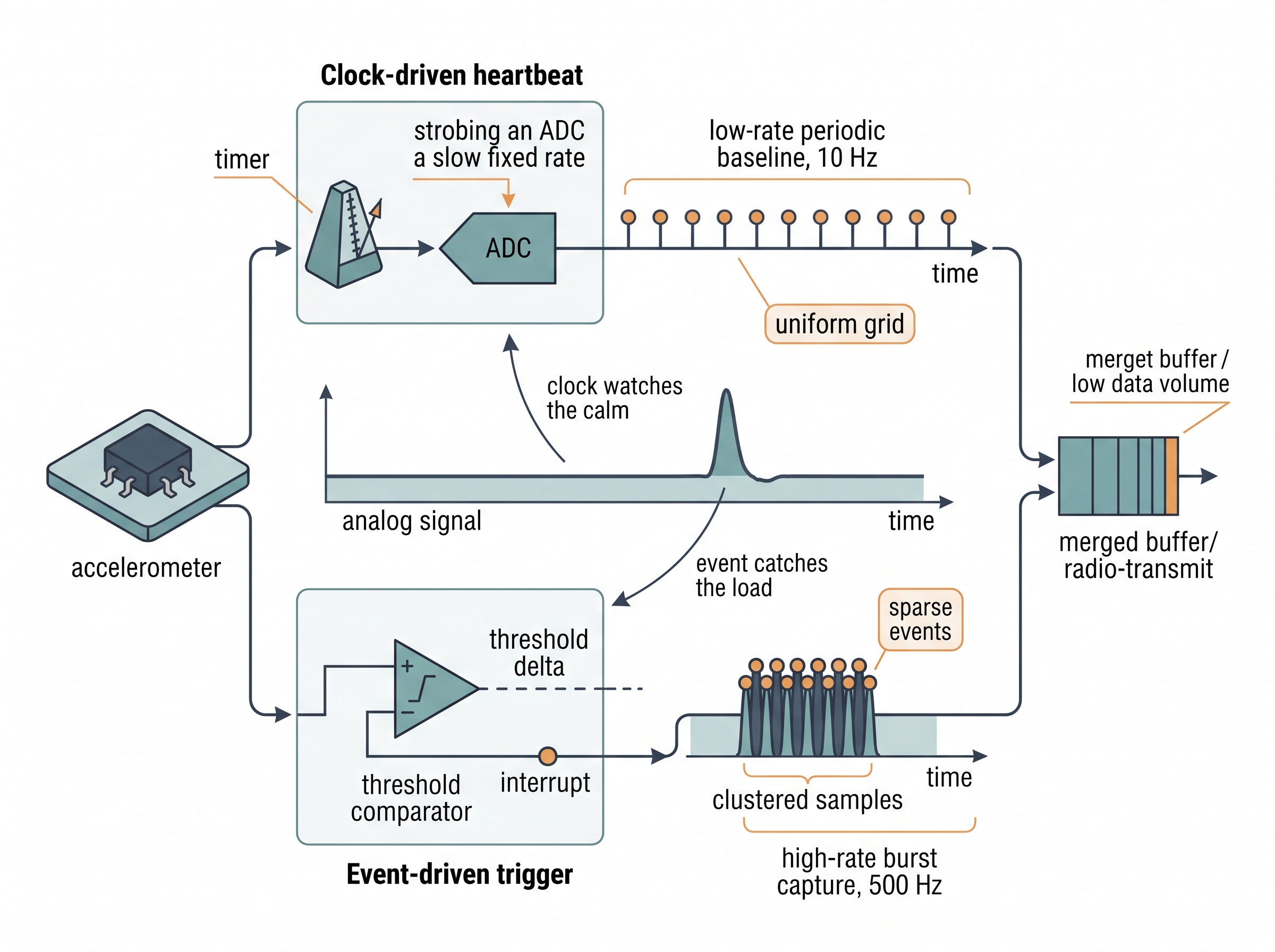
The common answer is both. Real systems hybridize. A wearable runs its accelerometer in low-rate periodic mode as a baseline and arms a high-rate interrupt that wakes a burst capture when motion spikes. The periodic stream gives context and clean features; the event trigger buys latency and detail without paying for them during the many quiet hours. That two-tier pattern feeds directly into the streaming-inference budgets of Chapter 60. Figure 3.2.1 illustrates Hybrid two-tier sensing architecture (periodic heartbeat plus amplitude-triggered event burst).

What's Next

Section 3.3 confronts the timestamps themselves. An event stream is only as trustworthy as the \(t_k\) on each sample. Reconcile several sensors, each on its own clock, into one timeline, and defining "the same instant" becomes the hard part of any multi-sensor system.