Quantization and compression

"Sampling decides when I get to look. Quantization decides how many answers the sensor is allowed to give. Compression decides how many of those answers survive the trip to me. I inherit whatever is left."

A Pragmatic AI Agent

A 24-bit accelerometer that reports only eleven honest bits is not defective. The other thirteen bits are amplifier hiss dressed up as data, and a downstream model will study that hiss as devotedly as the motion it was built to measure. This section therefore builds the amplitude story before the storage story. It leans throughout on the sampling picture from Section 3.1, the noise vocabulary of Chapter 2, and the information content that Chapter 4 makes precise. The two-stage path every sample takes, from continuous quantity to quantizer to compressed bitstream, is drawn in the figure below.

Amplitude quantization: a continuum forced onto a ladder

Get this ladder wrong and the damage is silent: a temperature logger with too-coarse steps will flatten a slow fever curve into a staircase and a fault-detection model will read those false plateaus as the physiology, learning an artifact of the converter instead of the patient. Everything downstream inherits the rungs you pick here. What it is. An \(N\)-bit converter with full-scale range \(V_{\text{FS}}\) partitions that range into \(2^N\) equal steps. Each step has width \(\Delta = V_{\text{FS}} / 2^N\), the value of the least significant bit (LSB). A true voltage \(v\) is reported as the nearest rung of this ladder, so the reading carries an error \(e = \hat v - v\) bounded by \(\pm \Delta/2\). Twelve bits over a \(\pm 2g\) accelerometer range give \(\Delta \approx 4g / 4096 \approx 0.001g\) per step: that is the finest distinction the sensor can express, no matter how quiet its analog front end.

Why it behaves like noise. For a signal that is busy relative to \(\Delta\) (it crosses many levels between samples), the rounding error \(e\) is well modeled as uniform on \([-\Delta/2, \Delta/2]\), independent from sample to sample. A uniform distribution of width \(\Delta\) has variance \(\Delta^2/12\), so quantization injects an effective noise power of \(\sigma_q^2 = \Delta^2/12\). This is the "quantization noise" that sets a hard floor: you cannot filter below it, because it was created at the moment of rounding and carries no structure to exploit.

How much resolution you actually buy. Comparing full-scale signal power to that noise floor gives the classic signal-to-quantization-noise ratio for a full-scale sinusoid:

Every added bit buys about 6 dB of headroom, roughly one extra factor of two in amplitude resolution. That single formula is the entire economics of bit depth: it tells you a 16-bit ECG channel tops out near 98 dB of dynamic range (the ratio between the largest and smallest amplitudes a channel can faithfully represent) on paper, and it warns you that if your analog noise already sits 40 dB below full scale, the bottom eight bits are just digitizing that noise. The honest resolution of a real channel is captured by its effective number of bits (ENOB), which folds analog noise and distortion back in and is almost always smaller than the nameplate \(N\). In short: a sensor's real resolution is written by its noise floor, not by the number stamped on the data sheet.

Dithering: the counterintuitive fix. When a signal is small relative to \(\Delta\), quantization stops looking like friendly noise and starts looking like distortion: a slow ramp gets rendered as flat plateaus with sudden stair-steps, and those steps are harmonically related to the signal, so they survive averaging and masquerade as real structure. Adding a tiny amount of noise (dither) of order \(\Delta\) before quantizing breaks the correlation, trading a visible staircase for a benign broadband hiss you can then average down. It feels wrong to add noise to reduce error, yet it is standard practice in audio and instrumentation converters for exactly this reason.

Non-uniform quantization: spend bits where the signal lives

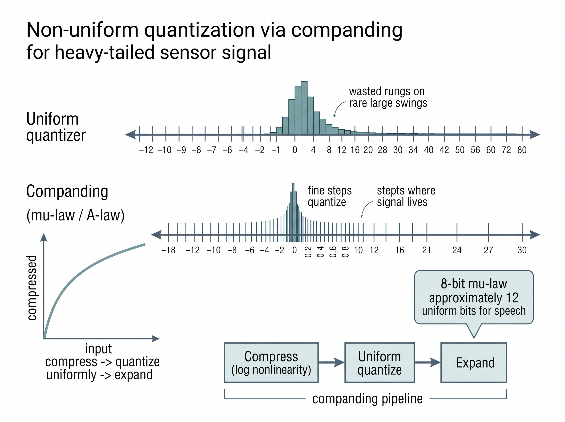
That headroom problem exposes a deeper inefficiency: the evenly spaced ladder we just built reserves as many rungs for the rare large swings near the rail as for the small values a signal spends most of its life inside, which is precisely the wrong way to spend a fixed bit budget.

What it is. A uniform ladder wastes resolution when the signal's amplitude distribution is heavy-tailed: most samples are small, yet a uniform quantizer reserves as many levels for the rare large excursions as for the common small ones. Non-uniform quantization allocates fine steps where samples are dense and coarse steps where they are sparse. The workhorse trick is companding: pass the signal through a compressive nonlinearity (logarithmic \(\mu\)-law or A-law in telephony), quantize the result uniformly, and expand on the far side. An 8-bit \(\mu\)-law channel delivers the perceptual dynamic range of roughly 12 uniform bits for speech, because human loudness perception is itself logarithmic, so four bits of the budget vanish for free the moment you place the levels on a log scale.

Why it matters for sensors. Many physical measurands share this heavy-tailed shape: vibration stays quiet then spikes at faults, and audio and photoplethysmography (PPG) run calm for long stretches between events. Placing quantization levels on a log or perceptual scale preserves small-signal fidelity where the interesting structure hides, yet still survives the rare large event without clipping. The cost is signal-dependent quantization noise, which any downstream calibration or uncertainty model must account for rather than assume a flat \(\Delta^2/12\). Figure 3.5.1 illustrates Non-uniform quantization via companding.

Compression: the same information in fewer bits

Quantization decided how many distinct values exist; compression decides how compactly the resulting stream of values is stored. Two families matter, and confusing them is a classic sensor-pipeline bug.

Compression re-encodes the same sample stream with fewer bits by removing what is predictable or perceptually irrelevant. It matters because radio bandwidth, storage, and battery bottleneck on-device sensors long before compute does. The mechanism models the data's statistics (a predictor for temporal redundancy, a transform for spectral redundancy) and then spends bits in proportion to surprise, so common patterns cost almost nothing and only rare deviations cost their full price. Reach for lossless when every bit must survive for correctness or audit (medical, metrology, forensic streams); reach for lossy only when a measured, bounded distortion is provably harmless to the downstream task.

Two families: lossless and lossy

Lossless compression reconstructs the exact integers you fed in. It exploits redundancy: successive sensor samples are highly correlated, so instead of storing each absolute value you store the small difference from a prediction (delta or linear-predictive coding), then hand those small residuals to an entropy coder (Huffman, arithmetic, or range coding) that spends few bits on the common near-zero residuals and more on the rare large ones. The entropy of the residual stream from Chapter 4 is the theoretical floor; FLAC does this for audio, and the same predict-then-entropy-code recipe typically compresses slowly varying industrial telemetry by three to five times with zero fidelity loss. Because it is exact, lossless compression never changes what a model sees; it only changes the bandwidth bill.

Lossy compression throws away information deemed unimportant to buy far larger savings: quantizing transform coefficients (as MP3 and JPEG do), dropping high-frequency detail, or downsampling. The ratios are dramatic (10x and beyond), but the discarded information is gone, and its absence is structured, not random. This is where sensor AI gets bitten.

The short simulation below makes the amplitude story concrete: it quantizes a sinusoid at several bit depths, measures the achieved SQNR, and checks it against the \(6.02N + 1.76\) prediction.

import numpy as np

def quantize(x, n_bits, v_fs):
    step = v_fs / (2 ** n_bits)                 # LSB width
    q = np.round(x / step) * step               # snap to nearest rung
    return np.clip(q, -v_fs / 2, v_fs / 2)      # respect the rails

t = np.linspace(0, 1, 20000, endpoint=False)
x = 0.5 * np.sin(2 * np.pi * 7 * t)             # full-scale sinusoid, V_FS = 1.0

for n in (4, 8, 12, 16):
    xq = quantize(x, n, v_fs=1.0)
    noise = xq - x
    sqnr = 10 * np.log10(np.mean(x ** 2) / np.mean(noise ** 2))
    print(f"{n:2d} bits: measured SQNR {sqnr:5.1f} dB   "
          f"predicted {6.02 * n + 1.76:5.1f} dB")

import numcodecs, numpy as np

samples = (x * 32767).astype(np.int16)          # 16-bit ECG-like stream
codec = numcodecs.Delta(dtype='i2')             # predict: store differences
blosc = numcodecs.Blosc(cname='zstd', clevel=5) # entropy-code the residuals
packed = blosc.encode(codec.encode(samples))
back = codec.decode(blosc.decode(packed))
assert np.array_equal(samples, back)            # exactly lossless
print(f"ratio: {samples.nbytes / len(packed):.1f}x")

What's Next

Section 3.6 assembles quantized, compressed sample streams into the units a model actually consumes: buffers, windows, and frames. Quantization and compression decided how faithful each sample is and how cheap it is to move; framing decides how those samples are grouped in time before they reach a feature extractor or a network, closing the loop from raw acquisition to model-ready tensors. The bit-budget decisions here also foreshadow the on-device tradeoffs of Chapter 59, where quantizing the model rather than the signal follows the very same 6-dB-per-bit logic.