Random variables, distributions, and moments for signals

"I reported the temperature as 21.4 degrees with the confidence of a stone tablet. Nobody asked me the one question that mattered: 21.4, plus or minus what?"

A Recalibrated AI Agent

We treat each sample as a random variable: a rule that assigns a number to the outcome of a random experiment, here the experiment being "let the transducer report once." A random variable \(X\) is described completely by its distribution, and for a real-valued sensor reading that distribution is captured by a probability density function \(p_X(x)\), where \(p_X(x)\,dx\) is the probability that a reading lands in the sliver \([x, x+dx]\). The density integrates to one, \(\int_{-\infty}^{\infty} p_X(x)\,dx = 1\), which says the sensor always returns something.

The probability density function \(p_X(x)\) is precisely a non-negative function whose integral over any interval gives the probability the reading lands in that interval; it is not itself a probability (its value can exceed 1) but a probability per unit of the measured quantity. It matters because it is the complete description of one continuous reading: every mean, variance, and alarm threshold you compute later is an integral taken against it. Mechanically it works by weighting outcomes so that dense regions of \(x\) accumulate more probability mass than sparse ones, and you recover any probability by integrating over the range you care about. Reach for the density when the reading is continuous and you want the full shape; switch to a probability mass function for discrete counts (a Poisson pixel), or to the cumulative form \(F_X(x)\) when all you need is "probability below a threshold."

From one sample to a random variable: what, why, and when

What changes when we call a reading a random variable is that we stop asking "what is the value?" and start asking "what values are plausible, and with what weight?" Why this matters for sensory AI is that the physical noise sources of Chapter 2, thermal agitation, quantization, shot noise, are themselves random processes, so the only faithful description of a reading is probabilistic. How we work with it is through two summaries that we can actually compute from data: the density (or its cumulative form \(F_X(x) = P(X \le x)\)) when we want the full picture, and a handful of moments when we want a compact fingerprint. When you can get away with just the moments rather than the full density is the recurring judgment call of this chapter, and the Gaussian case, where two moments are the whole density, is why the Gaussian shows up everywhere. That last judgment, how few moments you can safely keep, only sharpens once you know which distributions a sensor actually produces, so we meet the usual cast first.

The distributions that actually appear in sensor data

A small cast of distributions covers most of what a sensor stream throws at you, and each earns its place from a physical mechanism, not mathematical convenience.

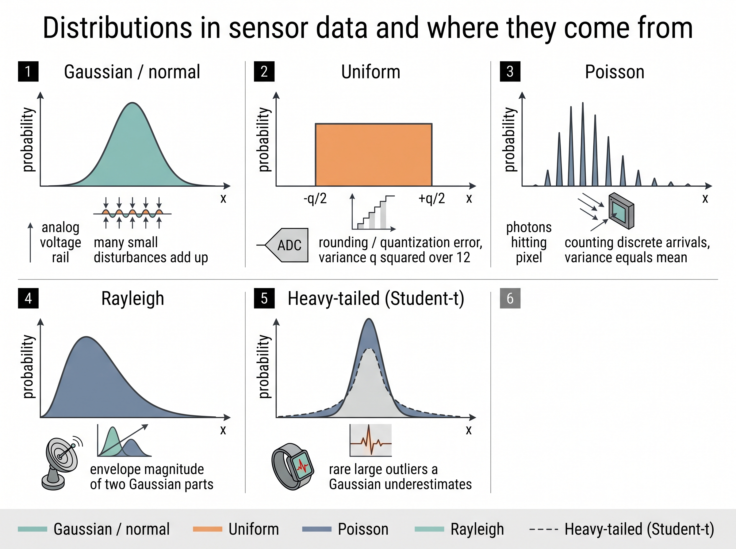
The Gaussian (normal) distribution, \(p(x) = \tfrac{1}{\sqrt{2\pi}\sigma}\exp\!\big(-\tfrac{(x-\mu)^2}{2\sigma^2}\big)\), dominates because of the central limit theorem (CLT): when many small independent disturbances add up, as they do in an analog front end, their sum tends toward a Gaussian regardless of the individual shapes. That is why we model thermal noise on a voltage rail as Gaussian, and why the Kalman filter of Chapter 9 can be optimal and cheap at the same time. The uniform distribution describes quantization error: an analog-to-digital converter (ADC) with step \(q\) rounds the truth, and the leftover error spreads flat across \([-q/2, q/2]\), giving the famous quantization-noise variance \(q^2/12\). The Poisson distribution counts discrete arrivals, photons hitting a pixel or ticks on a Geiger counter, so a photon-limited camera or lidar return is typically well modeled as Poisson. Its signal-dependent noise (variance equal to the mean) is why dark scenes look grainier.

The Rayleigh distribution appears whenever you take the magnitude of two independent Gaussian components, which is exactly the envelope of a radar or radio-frequency (RF) signal; it is the reason Chapter 44 reasons about detection thresholds probabilistically. Finally, heavy-tailed distributions (Student-t, log-normal) model the rare large outliers that a pure Gaussian badly underestimates, such as a motion spike from a footstep on a wearable. In short: a sensor reading is a distribution wearing the disguise of a single number, and its moments are how you see through the disguise. Figure 4.1.1 illustrates the distributions that appear in sensor data and their physical mechanisms.

Moments: the compact fingerprint of a distribution

Get the fourth moment wrong and the cost is not abstract: a fall detector cries wolf dozens of times a day, or a drone's estimator trusts a spiking accelerometer and tumbles out of the sky. The compact summaries below are what stand between a shipping device and those failures. Having just been warned to inspect the higher moments before trusting a two-number summary, we can now pin down exactly what those moments are. Moments are expectations of powers of the variable, where the expectation \(\mathbb{E}[\cdot]\) is just the probability-weighted average of a quantity over all outcomes, and the first four carry almost all the intuition you need. The mean \(\mu = \mathbb{E}[X] = \int x\,p(x)\,dx\) is the center of mass, the value a long average converges to; for a sensor it is the true signal plus any constant bias. The variance \(\sigma^2 = \mathbb{E}[(X-\mu)^2]\) is the spread, and its square root, the standard deviation \(\sigma\), lives in the same units as the reading, which is why we quote "plus or minus \(\sigma\)." The skewness \(\gamma_1 = \mathbb{E}[(X-\mu)^3]/\sigma^3\) measures asymmetry: a positive skew means occasional large-positive excursions, the signature of a rectified or count-based signal. The kurtosis \(\gamma_2 = \mathbb{E}[(X-\mu)^4]/\sigma^4\) measures tail heaviness; a Gaussian sits at exactly 3, and anything meaningfully above it warns you that rare large events happen more often than a Gaussian would predict, which is a direct input to how you set alarm thresholds and to the outlier-robust filters of Chapter 6. The moment ladder in Figure 4.1-1 traces this whole pipeline: a raw sample stream collapses into a density, and each successive moment reads off one more feature of that density's shape.

import numpy as np
from scipy import stats

# Simulated 100 Hz accelerometer: gravity bias + Gaussian noise + rare spikes
rng = np.random.default_rng(0)
n = 20_000
clean = 9.81 * np.ones(n)                       # true value (m/s^2)
noise = rng.normal(0.0, 0.05, n)                # thermal jitter, sigma = 0.05
spikes = rng.binomial(1, 0.002, n) * rng.normal(0, 1.0, n)  # rare footstep taps
x = clean + noise + spikes

print(f"mean      = {x.mean():.4f}")            # ~ 9.81, recovers the true value
print(f"std       = {x.std():.4f}")             # inflated above 0.05 by the spikes
print(f"skewness  = {stats.skew(x):+.3f}")      # near 0: spikes are symmetric
print(f"kurtosis  = {stats.kurtosis(x):+.3f}")  # >> 0 (excess): heavy tails, not Gaussian

The code makes the earlier point concrete: a clean Gaussian stream and the spiked stream report nearly the same mean and standard deviation, yet only the kurtosis reveals that one of them will throw values no Gaussian safety margin ever budgeted for.

Signals are sequences of random variables: joints, stationarity, and correlation

A single sample is a random variable; a signal \(x[0], x[1], \dots\) is a whole family of them, a random process. What ties the samples together is the joint distribution (the single probability rule governing several samples considered together, not one reading at a time), and the practical shortcut for describing it is the autocovariance \(C[k] = \mathbb{E}[(x[n]-\mu)(x[n+k]-\mu)]\), which measures how strongly a reading predicts one \(k\) steps later. Real sensor noise is rarely "white" (uncorrelated across time); a drifting gyroscope bias, for instance, produces samples that stay correlated for seconds. We usually assume wide-sense stationarity: the mean and autocovariance hold steady over time. That assumption lets us estimate those statistics by averaging along the stream, so we do not need many parallel sensors. When two channels are involved, say an accelerometer's three axes, the pairwise second moments assemble into a covariance matrix \(\Sigma\). Its off-diagonal entries reveal cross-axis coupling, and its structure feeds directly into the multivariate Gaussian that Chapter 9 propagates through time.

What's Next

In Section 4.2, we turn from describing distributions to inferring them from data. The moment estimates you computed above were guesses at unknown truths, and every guess has a bias and a variance of its own. We will formalize what makes an estimator good, expose the bias-variance tradeoff that governs every fit in this book, and derive maximum likelihood, the principled engine that turns a stream of samples into the best parameters for the distribution behind them.