Estimators, bias-variance, and maximum likelihood

"Every number I report is a guess with a track record. My job is to know how good the track record is before you trust the guess."

A Self-Aware AI Agent

This section assumes you are comfortable with random variables, expectation, and variance from Section 4.1, and with the sensor noise models introduced in Chapter 2. Everything here is frequentist: the parameter is a fixed unknown and the data is random. The complementary Bayesian view, where the parameter itself carries a distribution, arrives in Section 4.3.

What an estimator is, and how to grade one

An estimator \(\hat\theta\) is any function of the data \(X_1,\dots,X_n\) that we use to guess an unknown parameter \(\theta\). Because the data is random, \(\hat\theta\) is a random variable with its own distribution, called the sampling distribution. We grade an estimator by properties of that distribution, not by any single run.

The sampling distribution is precisely the probability distribution of the estimator \(\hat\theta\) taken over hypothetical repetitions of the entire experiment, each run supplying fresh random data. It matters because every quality we care about, bias, variance, and confidence intervals alike, is a feature of this distribution rather than of the one number you happened to compute. Mechanically you can approximate it without any repeated experiments through the bootstrap: resample your existing data with replacement many times, recompute \(\hat\theta\) on each resample, and read the spread off the resulting histogram. Reach for the sampling distribution whenever you need to attach honest error bars to a reported value; a lone point estimate carrying no sense of its own sampling distribution is a guess with no track record. Figure 4.2.2 illustrates the estimation pipeline: from noisy sensor data to a graded estimate via its sampling distribution.

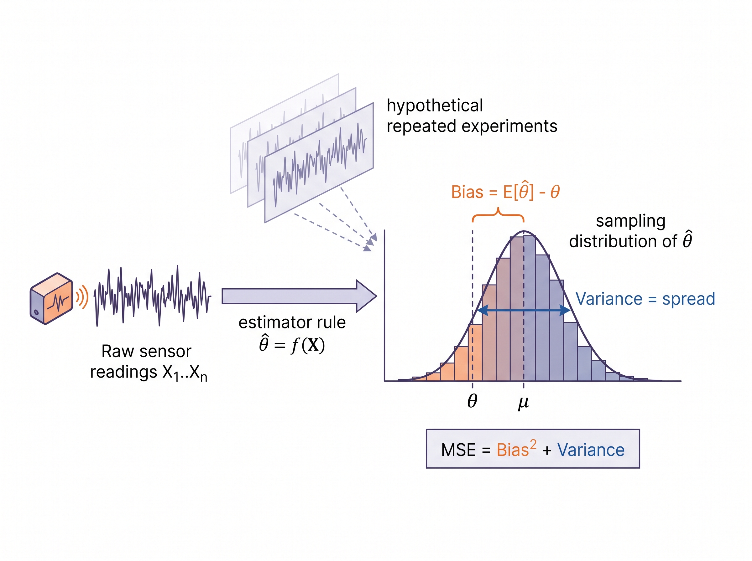
Bias measures systematic error: \(\operatorname{Bias}(\hat\theta) = \mathbb{E}[\hat\theta] - \theta\). An estimator is unbiased if, averaged over infinitely many experiments, it lands on the truth. Variance measures spread: how far a single estimate typically strays from its own average. The quantity that actually matters for a deployed system combines both, the mean squared error (MSE):

This identity is the spine of the whole section. It says total error has exactly two ingredients, and they trade against each other. A thermostat that always reads two degrees high has bias but no variance; a cheap sensor that jitters wildly around the true value has variance but no bias. Both are wrong, and MSE counts them on the same scale.

Consistency and efficiency

Two more properties matter in practice. An estimator is consistent if \(\hat\theta \to \theta\) as \(n\to\infty\): more data eventually crushes the error. It is efficient if, among unbiased estimators, it has the smallest possible variance. Consistency is the minimum bar for a sensor calibration routine; efficiency tells you whether spending money on a better algorithm can help, or whether you have already hit the physics-imposed floor. In short: an estimator is a promise made under uncertainty, and bias, variance, and Fisher information (defined later in this section, once we reach the Cramer-Rao bound) are the three numbers that tell you how much that promise is worth.

The bias-variance tradeoff as a design dial

The tradeoff is not an abstraction; it is a knob you turn every day. Consider estimating a slowly-drifting quantity, say the resting heart rate baseline of a wearer, by averaging the last \(n\) beats. A long window (large \(n\)) drives variance down like \(1/n\) because averaging cancels independent noise. But a long window also reaches back into stale data. If the true baseline is drifting, the average lags behind reality and picks up bias. A short window tracks the drift faithfully (low bias) but barely averages anything (high variance). There is an optimal window length that minimizes MSE, and it depends on the noise level and the drift rate. This same shape recurs in filter bandwidth choices in Chapter 6 and in model capacity choices for the neural sensor models of Chapter 13.

The model-complexity version is identical in spirit. A tiny model is too rigid to capture the signal, so it is biased (underfitting). A huge model bends to fit the noise in your particular training set, so it has high variance and generalizes poorly (overfitting). Every regularization technique, weight decay, dropout, early stopping, is a device for buying variance reduction with a controlled dose of bias. Figure 4.2.1 plots this decomposition directly: as complexity rises, squared bias falls while variance climbs, and their sum, the mean squared error, bottoms out at an intermediate optimum rather than at either extreme.

Maximum likelihood: one recipe for almost every estimator

Nearly every calibrated number a modern sensor system reports, from your phone's step count to a spacecraft's position fix, is produced by one estimation recipe; choose it badly and the error leaks silently into every downstream decision that trusts the reading. Where do good estimators come from? Most of the time, from maximum likelihood estimation (MLE). The recipe has three moves. Write down a probabilistic model \(p(x \mid \theta)\) for how your sensor produces data given the parameter. Given the actual data you observed, treat that probability as a function of \(\theta\), the likelihood \(L(\theta) = \prod_i p(x_i \mid \theta)\), and pick the \(\theta\) that makes the observed data most probable:

We maximize the log-likelihood because sums are numerically kinder than products and because the logarithm turns the exponentials in most noise models into tidy quadratics. Here is the payoff that connects a whole thread of the book: if your sensor noise is Gaussian, maximum likelihood is exactly least squares. Maximizing \(\sum_i \log p(x_i\mid\theta)\) for \(p = \mathcal{N}(\mu(\theta), \sigma^2)\) is the same as minimizing \(\sum_i (x_i - \mu(\theta))^2\). The sample mean, linear regression, and the Kalman filter update of Chapter 9 are all maximum-likelihood estimators under a Gaussian assumption in disguise.

MLE earns its dominance because, under mild conditions, it is asymptotically unbiased (unbiased in the limit of large sample size), consistent, and efficient: with enough data it reaches the lowest variance any unbiased estimator can achieve. That floor has a name.

Computing a maximum-likelihood estimate

With that floor now in hand as a yardstick, the natural next step is to compute an actual maximum-likelihood estimate and hold it up against the bound. Consider a common sensor-modeling task: your accelerometer sits still, and you want to estimate the noise standard deviation \(\sigma\) of its output so you can feed it to a downstream filter. Assume readings are Gaussian around a fixed (also unknown) bias \(\mu\). The code below fits both by maximum likelihood and compares against the Cramer-Rao lower bound on the variance of \(\hat\sigma\), so you can see whether your estimate is as good as physics allows.

import numpy as np

rng = np.random.default_rng(0)
true_mu, true_sigma, n = 0.02, 0.15, 500          # bias (g), noise std (g), samples
x = rng.normal(true_mu, true_sigma, size=n)        # a still accelerometer axis

# Maximum-likelihood estimates for a Gaussian: closed form.
mu_hat = x.mean()                                  # MLE of the mean
sigma_hat = x.std(ddof=0)                           # MLE of std (divides by n, biased low)
sigma_unbiased = x.std(ddof=1)                      # Bessel-corrected (divides by n-1)

# Cramer-Rao lower bound on Var(sigma_hat) for a Gaussian: sigma^2 / (2n).
crlb_var_sigma = true_sigma**2 / (2 * n)

print(f"mu_hat      = {mu_hat:+.4f}  (true {true_mu:+.4f})")
print(f"sigma_hat   = {sigma_hat:.4f}  MLE, biased low by ~sigma/(2n)")
print(f"sigma_unbi. = {sigma_unbiased:.4f}  (true {true_sigma:.4f})")
print(f"CRLB std of sigma_hat = {np.sqrt(crlb_var_sigma):.4f} g")

Notice the concrete appearance of bias-variance in the output: the plain MLE of \(\sigma\) is biased low (it divides by \(n\)), while the Bessel-corrected estimate is unbiased (it divides by \(n-1\)). At \(n=500\) the gap is tiny, which is exactly the point, the bias of MLE vanishes as data grows, so we tolerate it in exchange for the recipe's generality.

from scipy import stats
mu_hat, sigma_hat = stats.norm.fit(x)        # MLE, one line
df, loc, scale   = stats.t.fit(x)            # heavy-tailed? swap the family

When maximum likelihood misleads you

MLE is powerful, not infallible, and sensor data breaks its assumptions in predictable ways. First, model misspecification: MLE finds the best parameter within the family you assumed. If you assume Gaussian noise but your accelerometer occasionally emits large spike outliers, the fitted \(\sigma\) inflates to cover the spikes. Every downstream estimate then suffers. The remedy is a heavier-tailed likelihood (Student-t, Huber) so a few outliers no longer dominate. Second, small samples: MLE's beautiful efficiency is asymptotic, and with a handful of points it can be badly biased or even undefined. That is precisely the regime where borrowing strength from a prior pays off, which motivates the Bayesian treatment in Section 4.3. Third, MLE gives you a point estimate; it does not, by itself, tell you how much to trust that point. Quantifying that trust, and separating noise you cannot reduce from ignorance you can, is the subject of Section 4.4 on aleatoric versus epistemic uncertainty.

What's Next

In Section 4.3, we let the parameter carry a distribution of its own instead of treating it as a fixed unknown. Treating \(\theta\) as random turns the gas-sensor shrinkage trick into a principled framework, injects prior knowledge when data is scarce, and returns a full posterior we can propagate through the sensing pipeline rather than a lone point estimate.