Noise sources and signal-to-noise ratio

"Every reading I return is the truth plus an apology I never asked to write."

A Self-Aware AI Agent

This section assumes the resolution, sensitivity, and dynamic-range vocabulary from Section 2.2, plus random variables, variance, and expectation. If those feel shaky, the Probability, Estimation, and Uncertainty Primer (Chapter 4) makes the statistics here rigorous. We stay physical and definitional: what the noise is, why it is there, and how to measure it.

Where the noise comes from

Noise is any component of the sensor output that does not correspond to the observable you intend to measure. It is useful to sort noise by its physical origin, because origin dictates behavior: how it scales with signal, temperature, and bandwidth, and therefore how you can fight it. Figure 2.3.1 lays out this noise budget: several independent physical sources sum into a single noise floor, and the gap between that floor and the signal power is the SNR we define later in the section.

Thermal (Johnson-Nyquist) noise is the voltage jitter produced by charge carriers rattling around in any resistive element at non-zero temperature. Its mean-square noise voltage is \(\langle v_n^2 \rangle = 4 k_B T R \, \Delta f\) (the available noise power delivered to a matched load is \(k_B T \, \Delta f\), independent of \(R\)), so it grows with temperature \(T\), resistance \(R\), and measurement bandwidth \(\Delta f\). It is white (flat across frequency) and unavoidable above absolute zero, which is why cooled detectors and narrow bandwidths are the two classic weapons against it.

Shot noise arises because signals are quantized into discrete carriers: electrons across a junction, photons hitting a pixel. When you count \(N\) discrete events, the count fluctuates with standard deviation \(\sqrt{N}\) (Poisson statistics, the counting statistics of independent, randomly timed events). This is why a photodiode in bright light has more absolute noise but better relative noise than in dim light, and why low-light imaging is fundamentally hard.

Device and environmental noise

Flicker (1/f) noise has a power spectral density (how noise power is distributed across frequency) that rises at low frequencies. It dominates slow measurements and direct-current (DC) coupled sensors, and it is the reason a temperature probe left untouched still wanders over minutes. Quantization noise is the rounding error the analog-to-digital converter injects when it snaps a continuous voltage to the nearest code; we treat it in depth alongside sampling in Signals, Sampling, Time, and Synchronization (Chapter 3). Layered on top are environmental and interference terms: 50/60 Hz mains pickup, motion artifact in a wrist sensor, electromagnetic coupling from a nearby motor. In short: name each noise source by its physics, quote the ratio it leaves behind, and you have already set the ceiling on everything a downstream model can recover.

Defining signal-to-noise ratio

Ship a heart-rate algorithm tuned on clean bench data and it can fail outright on a drugstore chest strap, not because the code is wrong but because the measurement feeding it is a fraction as clean; the number that predicts that failure in advance is the one we define next. With the individual noise sources named and sorted by color, the next job is to fold their combined effect into a single figure of merit. SNR compresses "how clean is this measurement" into one number: the ratio of signal power to noise power,

Because power is amplitude squared, an SNR expressed from amplitudes uses \(20 \log_{10}(A_\text{signal}/A_\text{noise})\). The decibel scale is logarithmic, so every 10 dB is a factor of ten in power, every 3 dB roughly a doubling. As a feel for the numbers: a clean lab-grade measurement might sit at 60 to 80 dB, a wearable photoplethysmogram on a moving wrist can drop below 6 dB during exercise, and detection near 0 dB means signal and noise carry equal power (a coin flip without further processing). (That span from a lab bench to a moving wrist is a collapse of ten thousand to a million times in signal-to-noise power, which is why a model that shines on clean data can fail outright on a wearable.)

Two cousins deserve names. The noise floor is the output you see with no input signal present, and it sets the smallest change you can resolve. The minimum detectable signal is the input that produces an output equal to the noise floor, conventionally where SNR reaches 1. A sensor's usable dynamic range from Section 2.2 is bounded below by this floor and above by saturation, a ceiling we treat in Section 2.4.

Concretely, the noise floor is the root-mean-square (RMS) level of the sensor's output when you hold the input at zero. Express it in the same units as the signal: volts, counts, or, for spectra, volts per root-hertz. It matters because it is the hard boundary between a reading you can trust and one you are inventing. Any change smaller than the floor is indistinguishable from the sensor's own restlessness, so it directly fixes resolution and minimum detectable signal. Mechanistically it is nothing more than the summed variance of every noise source above, referred back to the input. Quote it as a single RMS number when your signal sits in a known fixed bandwidth. Switch to a spectral-density curve when the signal's band can move, since one flat total figure can hide a tall 1/f corner exactly where a slow measurement lives.

Measuring and improving SNR in practice

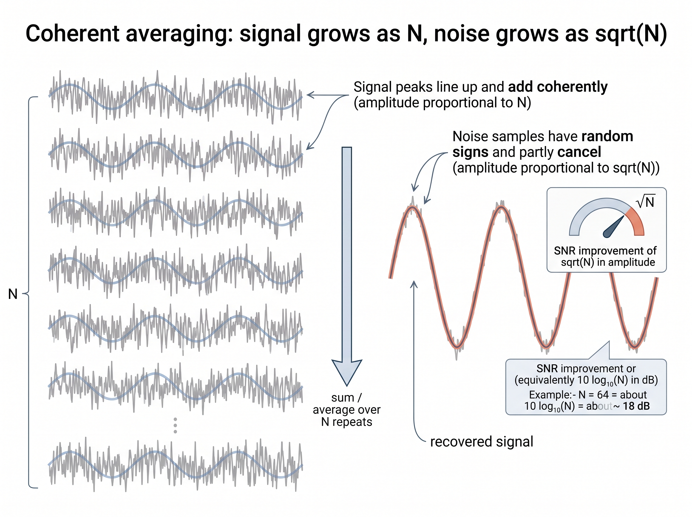
Having watched a real device rearrange its measurement to dodge noise, we can now name the general levers and quantify how much SNR each one buys. The single most reliable lever is coherent averaging. If you repeat a measurement \(N\) times with independent, zero-mean white noise, the signal adds coherently while the noise adds in quadrature (adding in quadrature means independent noise powers sum, so the amplitudes combine as the square root of the sum of squares rather than linearly). Amplitude SNR therefore improves by \(\sqrt{N}\): a 100-fold repeat buys 10x amplitude SNR, or 20 dB. This is the workhorse behind lock-in amplifiers, averaged evoked potentials, and multi-frame image stacking. It only works when the noise is white and the signal is stationary across the repeats. Colored noise and drift violate exactly that assumption. Other levers include narrowing bandwidth to the band the signal actually occupies (thermal noise power scales with \(\Delta f\)), matched filtering when the signal shape is known, and cooling the front end. Figure 2.3.1 illustrates Coherent averaging: signal adds linearly, white noise adds in quadrature (root-N SNR gain).

To estimate SNR from real data you separate a clean-signal estimate from a residual and compare their variances. The snippet below simulates a sine buried in white noise, recovers SNR, and demonstrates the \(\sqrt{N}\) averaging gain.

import numpy as np

rng = np.random.default_rng(0)
fs, f0, T = 1000, 5.0, 2.0           # sample rate, tone freq, duration
t = np.arange(0, T, 1/fs)
clean = np.sin(2*np.pi*f0*t)         # the observable we want
noise_sigma = 1.5                    # white noise standard deviation

def snr_db(sig, noisy):
    resid = noisy - sig
    return 10*np.log10(np.var(sig) / np.var(resid))

single = clean + rng.normal(0, noise_sigma, t.size)
print(f"single-shot SNR:  {snr_db(clean, single):5.1f} dB")

N = 64                               # coherent averaging over N repeats
stack = np.mean([clean + rng.normal(0, noise_sigma, t.size)
                 for _ in range(N)], axis=0)
print(f"averaged (N={N}): {snr_db(clean, stack):5.1f} dB")
print(f"predicted gain:   {10*np.log10(N):5.1f} dB")

Why SNR is the ceiling for AI

A learned model cannot recover information the measurement never contained. Once signal and noise overlap in the feature the model relies on, no architecture, however large, can separate them with certainty; it can only report a calibrated probability (a confidence value tuned to match the true long-run frequency of being correct). SNR therefore sets an information-theoretic ceiling on accuracy, and the honest job of a model near that ceiling is to quantify its own uncertainty rather than hallucinate confidence. That is why sensor-facing systems pair predictions with uncertainty, a thread that runs from the estimation foundations in Chapter 4 through calibration and conformal methods (Chapter 18) later in the book. A practical corollary: reporting the SNR of your training data is as important as reporting the model, because a benchmark collected at 40 dB tells you nothing about deployment at 5 dB.

What's Next

In Section 2.4, we turn from the random part of the error to its structured, repeatable part: bias, drift, hysteresis, and saturation. These are the errors that do not average away and that a naive noise model will silently absorb into the wrong place, and understanding them completes the measurement-error picture before we assemble the full transfer function.