Bias, drift, hysteresis, saturation

"Noise I can average away. Bias just lies to me politely, drift lies a little more each day, hysteresis lies about where it has been, and saturation stops answering the question entirely."

A Weary AI Agent

A pulse oximeter that reports a steady but wrong oxygen level, or a gyroscope whose zero creeps as it warms, can pass every repeatability test and still send a model quietly off the rails; these systematic errors are the ones no amount of extra data can cure, and mistaking them for noise is how field deployments fail. Recall the measurement model from Chapter 1, \(x = h(s) + \eta\). Section 2.3 put all sensor imperfection into \(\eta\) and showed how to beat it down with signal-to-noise ratio. That framing hides a trap: it suggests every error is zero-mean and independent, so more data always helps. It is not, and it does not. The four phenomena in this section are deformations of \(h\) with structure and memory. You need only functions, a little calculus, and the probability intuitions that Chapter 4 makes rigorous. We take each in turn, name its fingerprint, and say what to do about it.

Bias: a constant lie

What it is. Bias (also called offset) is a constant additive error. The response is really \(x = h(s) + b + \eta\), where \(b\) does not depend on the state \(s\) or on time. A scale that reads 0.3 kg with nothing on it has a bias of 0.3 kg; every reading is inflated by the same amount.

Precisely, bias is the fixed component of error that remains after the random part averages to zero. It shows up as a nonzero mean of the residual \(x - h(s)\) (the reading minus the ideal noise-free response), taken over many readings at a fixed state. It matters because it is the one error mode that more data cannot touch: every additional sample carries the same \(b\), so the sample mean converges to the truth plus \(b\), never to the truth. Mechanically it arises from a shifted reference point, a miswired zero, a thermal offset in the front-end electronics, or an aging component, all of which displace the whole response curve vertically. Reach for a bias correction (a tare or zero step) when the offset is stable over your measurement window; if it wanders, you need the drift machinery of the next subsection instead.

Why it earns its own name. Because it survives everything you would normally do to clean a signal. It is not zero-mean, so time-averaging preserves it exactly; it is not high-frequency, so a low-pass filter passes it straight through. Bias attacks accuracy (closeness to truth) while leaving precision (repeatability) untouched, so a biased sensor can look reassuringly stable and be reliably wrong. In estimation terms it inflates the estimator bias while doing nothing to variance, which is exactly the axis that more samples cannot fix. In short: the errors worth naming are the ones that survive averaging, so you model them into the estimator rather than hope more data washes them out.

How to handle it. Measure it and subtract it. A one-time calibration under a known reference (a zeroing step, a tare) yields \(\hat b\), and you report \(x - \hat b\). The whole reason zeroing a scale before weighing works is that bias is stationary: what you measure at reference time still holds at measurement time.

Drift: bias that will not sit still

What it is. Drift is bias that changes slowly with time, temperature, or age: \(b \to b(t)\). Two flavors dominate. Deterministic drift follows a trend, often roughly linear, \(b(t) \approx b_0 + \beta t\), as a chemical electrode ages or a component warms up. Stochastic drift is a random walk, \(b(t{+}1) = b(t) + w_t\) with small independent steps \(w_t\); it has no trend to extrapolate, yet it wanders unboundedly far given enough time.

Why it is worse than bias. A one-time calibration expires: the \(\hat b\) from this morning is stale by afternoon, and for the random-walk kind, without bound. Hence recalibration schedules, and hence hopeless uncorrected inertial navigation: integrating a drifting gyroscope bias turns a tiny rate error into a linearly growing angle error, and then, because that heading error feeds a sideways velocity component that is integrated a second time into position, a position error that grows as time squared.

Hysteresis: the sensor remembers where it came from

Drift gave the error a memory of time; the next failure mode gives it a memory of path, a dependence not on when you measured but on how the input arrived at its current value.

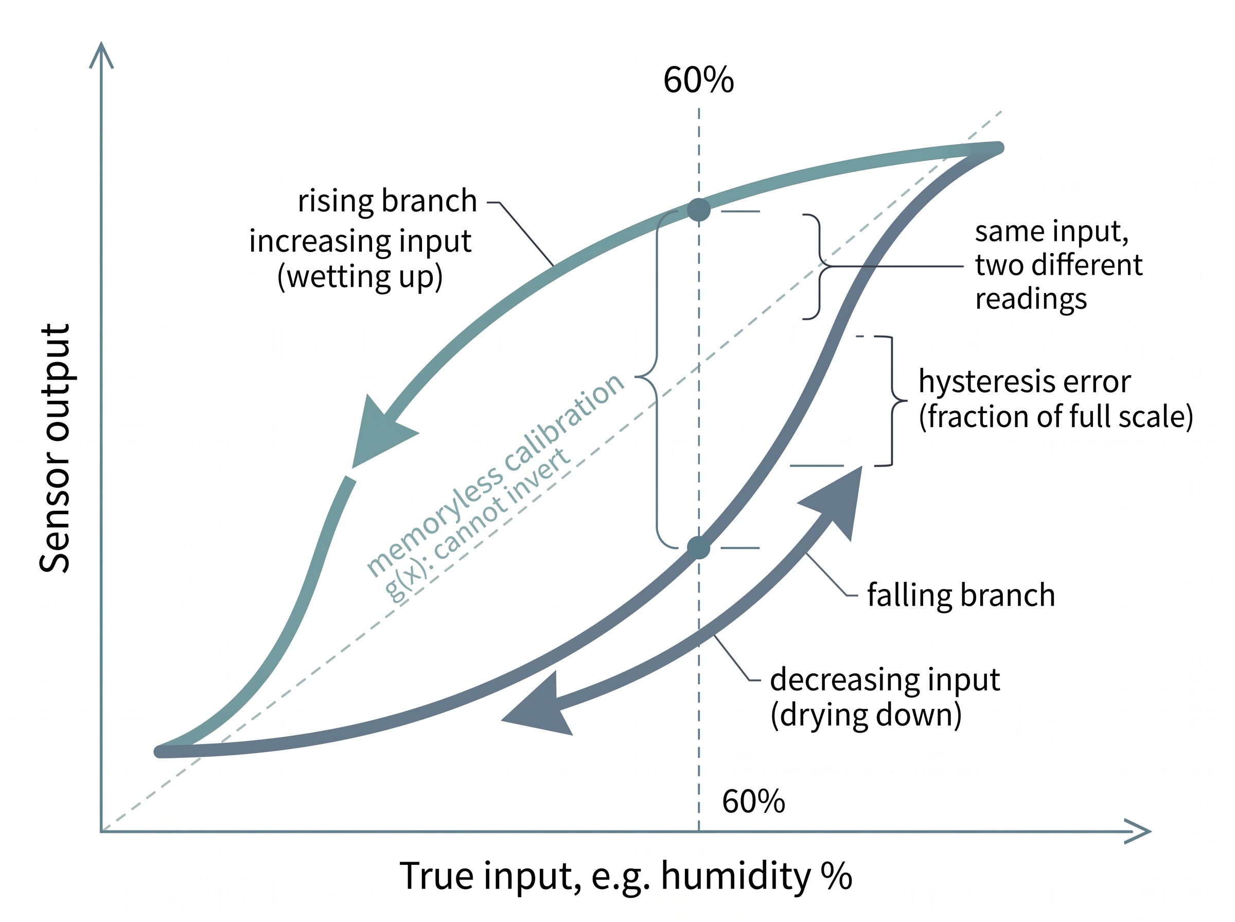
What it is. Hysteresis is path dependence: the output at a given state \(s\) differs depending on whether \(s\) was approached from below or from above. Plot output against a slowly rising-then-falling input and you get a loop, not a line. Ferromagnetic sensors, many humidity sensors, mechanical strain gauges, and any component with internal friction or material relaxation show it. The gap between the rising and falling curves, expressed as a fraction of full scale, is the hysteresis error.

Why it breaks naive correction. Bias and even drift are functions the current input can undo, but hysteresis makes the output a function of the input's history. No single number inverts it, and no memoryless calibration curve \(g(x)\) does either. Two different true states legitimately produce the same reading. A humidity sensor climbing from 30% to 60% and one falling from 90% to 60% can both display 58%. Any correction has to know the direction of travel. That requires memory, which pushes you again toward a stateful model rather than a lookup table. In practice you handle it by making the correction direction-aware: track whether the input is rising or falling and apply the matching branch of the loop, or fit an explicit hysteresis model (such as a Preisach or play operator) that carries the needed memory of past excursions. Figure 2.4.2 illustrates a hysteresis loop and path dependence.

Saturation: when the sensor stops listening

Hysteresis at least keeps answering, if ambiguously; the last failure mode is the one where the sensor stops answering altogether once the input pushes past the edge of its range.

What it is. Every real sensor has a finite range (revisit Section 2.2 on dynamic range). Past the top or bottom of that range the response flattens: the output clips at \(x_{\max}\) no matter how large the true state grows. Formally \(x = \min(h(s), x_{\max})\) at the top rail, with the analogous floor at the bottom. An accelerometer rated to \(\pm 16g\) reports \(16g\) for a \(40g\) impact, and reports it with perfect, useless steadiness.

Why it is uniquely dangerous. Saturation destroys information rather than distorting it, and it does so silently. A clipped reading is not merely inaccurate; it is censored, an inequality (\(s \ge s_{\text{sat}}\)) masquerading as an equality. Worse, saturation is most likely exactly when the state is most extreme, which is often exactly when it matters most: the crash sensor rails out during the crash, the microphone clips during the gunshot, the current sensor pins during the fault. A model trained on nicely-in-range lab data has never seen the flat top and will read it as a genuine plateau. The honest response is to flag saturated samples as censored and let downstream inference treat them as bounds, a theme Chapter 5 picks up with missing and corrupted data.

Seeing all four in one signal

These distortions rarely arrive alone. Before stacking them in code, it helps to fix each one's visual signature in mind. The four panels of Figure 2.4.1 plot each failure mode as sensor output (solid) against the true measurand (dashed), so bias reads as a parallel gap, drift as a widening wedge, hysteresis as a loop, and saturation as a flat rail. The short simulation below then stacks bias, linear-plus-random-walk drift, and hard saturation onto a clean sinusoid so you can watch each fingerprint appear. It is the seed of Lab 2, where you will quantify how each one degrades a classifier and an anomaly detector.

import numpy as np
rng = np.random.default_rng(0)
t = np.linspace(0, 20, 2000)
s = 3.0 * np.sin(0.5 * t)              # clean measurand h(s)

bias  = 0.8                            # constant offset b
drift = 0.05 * t                       # deterministic ramp
drift += np.cumsum(rng.normal(0, 0.01, t.size))   # random-walk drift
noise = rng.normal(0, 0.10, t.size)    # ordinary zero-mean noise

x = s + bias + drift + noise           # systematic errors do NOT average away
x_sat = np.clip(x, -3.5, 3.5)          # saturation: censors the extremes
censored = (x_sat != x)                # flag saturated samples as bounds

print(f"true mean {s.mean():+.3f}   observed mean {x_sat.mean():+.3f}")
print(f"samples lost to saturation: {censored.sum()} of {t.size}")

from filterpy.kalman import KalmanFilter
kf = KalmanFilter(dim_x=2, dim_z=1)    # state = [signal, slow bias]
# ... set F, H, Q (small on bias), R once ...
for z in x_sat:                        # skip z where censored[k] is True
    kf.predict(); kf.update(z)         # kf.x[1] is the tracked drift estimate

What's Next

Section 2.5 formalizes the response \(h\) itself as a transfer function and characterizes how fast a sensor reacts: rise time, settling time, and the lag that turns a sharp real event into a smeared reading. Bias, drift, hysteresis, and saturation deform what the sensor reports; response time governs when it reports it, and the two together complete the static-plus-dynamic picture of \(h\) that the rest of the book inverts.