Clocks, timestamps, and multi-sensor synchronization

"Each of my sensors swears it knows the time. The trouble is that no two of them agree, and none of them will admit it."

A Multi-Sensor AI Agent

Section 3.1 treated a single stream sampled on a single clock, and Section 3.2 contrasted clock-driven with event-driven acquisition. This section assumes the readings exist and asks the question fusion forces: how do we place samples from independent devices on a common axis? This presumes a little probability vocabulary for talking about timing error, which the Chapter 4 uncertainty primer supplies, and it feeds directly into Chapter 48, where misalignment becomes fusion error you can measure.

What a clock actually is: offset, skew, and drift

Get the clock model wrong and no downstream fix can rescue you: a rig of perfectly good sensors will smear its own data the moment one counter runs a hair fast, and the damage looks exactly like the bad calibration you will chase for weeks before suspecting time. A sensor's clock is a counter driven by an oscillator, usually a quartz crystal, that ticks at a nominal frequency. It is never exactly right. We model device \(i\)'s reported time \(C_i\) as an affine function (a straight-line map: a constant scaling of the input plus a constant shift) of true time \(t\):

Here \(\theta_i\) is the offset (how far the clock is ahead or behind at \(t=0\)) and \(\epsilon_i\) is the skew (its fractional rate error, the reason it gains or loses time). Skew is quoted in parts per million (ppm): a garden-variety consumer crystal is rated at \(\pm 20\) to \(\pm 50\) ppm. That sounds negligible until you unpack the unit. One ppm is one microsecond of error per second, which is about \(86\ \mathrm{ms}\) per day. A 50 ppm crystal can therefore drift more than four seconds in a single day if left uncorrected. Two independent 50 ppm clocks can move apart at up to 100 ppm relative to each other. Drift is the slow change of \(\epsilon_i\) itself, driven mostly by temperature. The same crystal that reads 20 ppm on a bench can swing tens of ppm as a device warms in a pocket or a bearing housing.

The practical takeaway is that offset and skew are not one-time nuisances you subtract once. Offset must be re-estimated because clocks are set imperfectly; skew must be re-estimated because a fixed rate error accumulates without bound; and drift means both estimates go stale, so synchronization is a process you run continuously, not a calibration you do at the factory. In short: a shared timebase is never measured, only estimated and re-estimated, because every clock you own is quietly lying at its own rate.

Where a timestamp really comes from

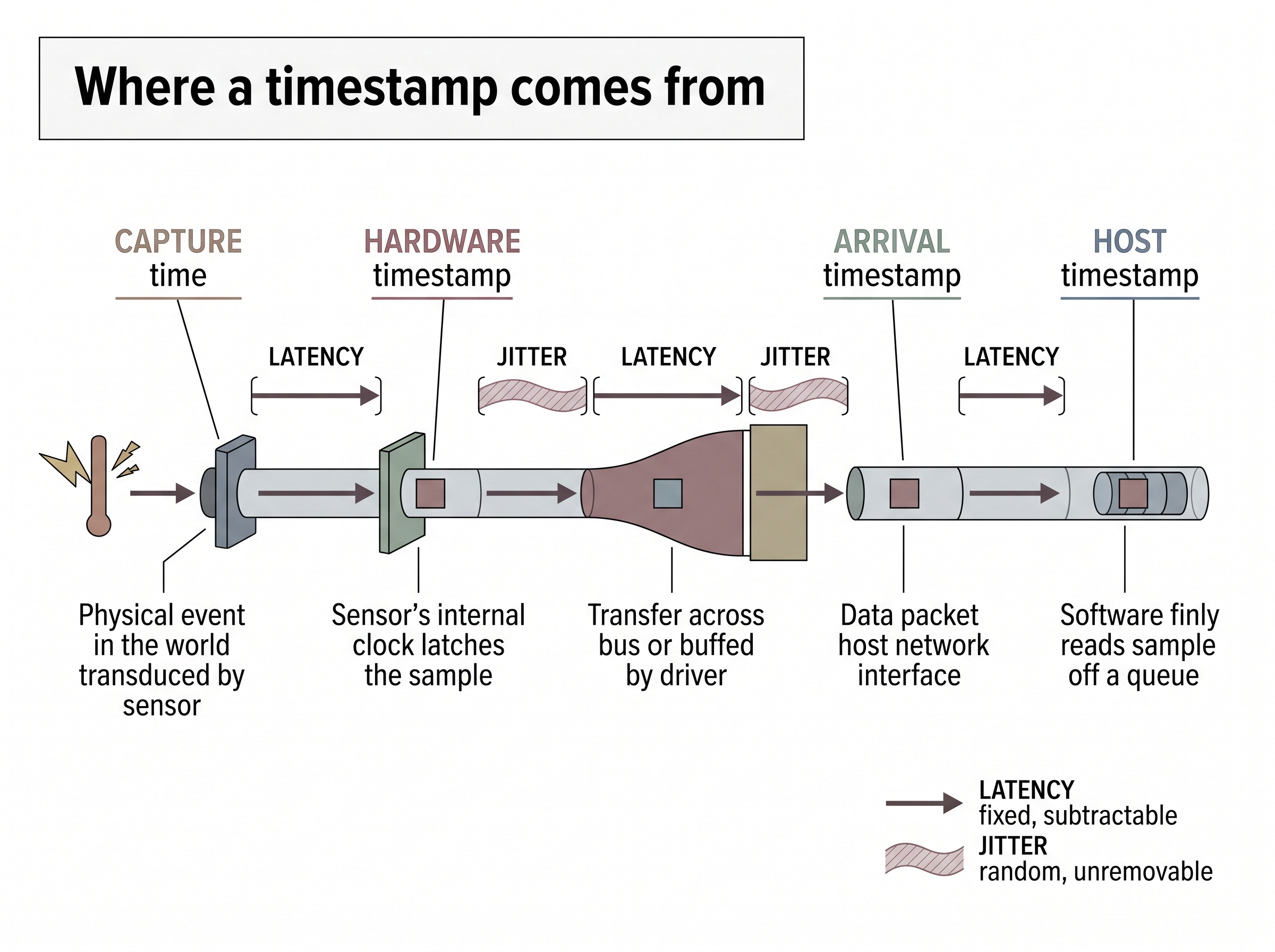
Fitting that line assumes the paired timestamps you feed it are trustworthy, which raises the prior question of where a timestamp actually comes from. A single sensor sample can carry several different timestamps, and confusing them is among the most common synchronization bugs in practice. A reading acquires its capture time when the physical event is transduced, a hardware timestamp if the sensor's own clock latches the sample, an arrival timestamp when the packet reaches the host, and a host timestamp when your software finally reads it off a queue. Between capture and host there is exposure time, bus transfer, driver buffering, and operating-system (OS) scheduling, and each adds a delay that is partly fixed and partly random. The fixed part is latency; the random part is jitter, treated as a failure mode in its own right in Section 3.4. Figure 3.3.1 illustrates the lifecycle of a single sample's timestamps: capture, hardware, arrival, and host times, and the latency and jitter accumulating between them.

The rule that saves projects is: timestamp as close to the physical event as the hardware allows, and record which clock did it. A camera that exposes a hardware timestamp at the middle of its integration window is worth far more than one you stamp when the Universal Serial Bus (USB) frame lands, because the arrival time smears the true capture instant by a variable few milliseconds. On the software side, always separate the monotonic clock (a counter that only ever increases, immune to being reset) from the wall clock (calendar time, which can jump backward when NTP (the Network Time Protocol, detailed below) corrects it or a leap second (an occasional one-second adjustment that keeps UTC in step with Earth's rotation) lands). Use the monotonic clock to measure durations and align streams; use the wall clock only to label data with human-readable dates. Mixing them produces negative time intervals and reversed sample orders that are maddening to debug.

Mechanisms that pull sensors onto one clock

That road-bending failure was cured in the timing layer with a hardware trigger, but such heavy machinery is overkill when sensors need only loose agreement, so it helps to survey the full range of options before committing to one. There is a ladder of synchronization techniques, and the right rung depends on how tightly your sensors must agree. Figure 3.3.1 lays out that ladder from loosest to tightest, pairing each mechanism with the order of agreement it buys. From loosest to tightest:

Network Time Protocol (NTP) disciplines a host's wall clock over an ordinary network to within a few milliseconds on a local area network (LAN), tens of milliseconds over the internet. It is enough to correlate slow logs and timestamp events for humans, and nowhere near enough to fuse a 100 Hz inertial measurement unit (IMU) with a camera. Precision Time Protocol (PTP, IEEE 1588) uses hardware timestamping in the network interface to exchange delay-measurement messages and reach sub-microsecond agreement across devices on the same switched network; it is a backbone of many synchronized industrial and automotive sensor buses. GPS with a pulse-per-second (PPS) signal gives every receiver a physical electrical edge aligned to Coordinated Universal Time (UTC) to within tens of nanoseconds, which is why GPS-disciplined clocks anchor large outdoor multi-sensor rigs and are covered further in Chapter 25. A hardware trigger is the tightest of all: one electrical line fires multiple sensors at the same instant, so they share not just a clock but a common exposure event, eliminating offset by construction.

NTP deserves a closer look, because you inherit it whether or not you plan for it: it runs on essentially every networked machine, so its accuracy is the clock quality you start from. The protocol repeatedly asks a set of time servers for the current time, records four timestamps per exchange (send and receive at each end), and slews (gradually adjusts the rate rather than jumping) the local wall clock to minimize the estimated offset. Assuming a symmetric network path, it splits the round trip to recover one-way delay and offset. Reach for NTP when a few milliseconds over a routed network suffices (correlating logs, tagging coarse events); step up to PTP or a hardware trigger the moment fusion needs sub-millisecond alignment, because NTP's symmetry assumption breaks down exactly where tight fusion lives.

When you cannot rewire the hardware, you fall back to post-hoc software alignment: record the best timestamps you have, then estimate the residual offset from the data itself. If two sensors observe the same physical event (a shake felt by two IMUs, an audio-visual clap), the lag that maximizes their cross-correlation (a measure of how well two signals overlap as one is slid in time past the other) is a direct estimate of \(\theta_i - \theta_j\). This is cheap, requires no special hardware, and is the workhorse for aligning consumer devices that were never designed to be synchronized. It cannot fix skew on its own, though, so for long recordings you fit the full affine map, not just a constant shift.

import numpy as np

# Paired timestamps: each row is (sensor_clock_reading, reference_clock_reading)
# gathered whenever a shared event let us observe both clocks at once.
sensor = np.array([0.001, 1.002, 2.004, 3.005, 4.007, 5.008])   # device clock (s)
ref    = np.array([0.000, 1.000, 2.000, 3.000, 4.000, 5.000])   # reference clock (s)

# Fit ref = a * sensor + b  (a undoes skew, b undoes offset)
A = np.vstack([sensor, np.ones_like(sensor)]).T
(a, b), *_ = np.linalg.lstsq(A, ref, rcond=None)

skew_ppm = (a - 1.0) * 1e6
print(f"skew = {skew_ppm:6.1f} ppm, offset = {b*1e3:6.2f} ms")

# Map any future device stamp onto the reference timeline:
def to_reference(device_stamp):
    return a * device_stamp + b

The code above is the whole idea in a dozen lines: gather pairs of readings taken at the same real instant, fit a line, and reuse it. In production you re-fit this map on a sliding window so it tracks drift rather than freezing a stale skew estimate.

import pandas as pd
# imu, cam: DataFrames sorted by a common-timeline column "t"
aligned = pd.merge_asof(cam, imu, on="t",
                        direction="nearest",
                        tolerance=0.005)   # drop pairs > 5 ms apart

The timestamp contract: what to record so alignment stays possible

Synchronization is only recoverable if you preserve the information it needs. This is a data-engineering discipline as much as a signal one, revisited under leakage-safe pipelines in Chapter 5. Every sample should carry: the timestamp value, the clock domain it came from (monotonic versus wall, and which device), and ideally the stamping stage (capture, hardware, or arrival). Store timestamps at nanosecond resolution in integer counts, not 32-bit floats, because a float32 second-count loses millisecond precision within an hour of uptime. Never overwrite a hardware timestamp with a host one to "clean up" the record; you are destroying the very evidence a later alignment step depends on. If you log the delay-measurement exchanges from PTP or the PPS edges from GPS, you can reconstruct and audit the timebase after the fact. That is the difference between a dataset that can be re-synchronized and one that is permanently smeared.

What's Next

Section 3.4 confronts what happens when the timeline you just built develops holes: samples that never arrive, timestamps that jitter around their true instant, and packets lost in transit. Clean synchronization assumes every sample is present and stamped; the next section drops that assumption and shows how to detect, mark, and reason about the gaps without letting them poison a downstream model.