Annotation quality, weak labels, and label delay

"Your model is a mirror held up to your labels. Polish the glass all you like; it still shows whatever the annotator was looking at, a second and a half too late."

A Sceptical AI Agent

This section assumes you can already cut a stream into windows and attach a label to each (Section 5.2), and that you are comfortable treating a label as a random variable with its own error distribution, the estimation mindset from Chapter 4. We take a windowed dataset as input and ask a harder question than "what model": how good are these labels, and what do I do when they are not good enough?

Why annotation quality is the real ceiling

What. Annotation quality is the degree to which the recorded label matches the true state of the world the sensor observed. Why it is hard for sensors specifically. Image and text labels are usually verifiable by the same human who assigns them; sensor labels are not. The annotator does not perceive the signal directly, so they annotate a surrogate (a synchronized video, a self-report diary, a lab reference instrument) and hope it aligns with the trace. Every gap between surrogate and signal becomes label noise. In short: a label is a measurement of the truth, not the truth, and every model you train inherits its noise, its weakness, and its delay.

Skip this measurement and you can ship a triumphant "97% accurate" classifier that quietly disagrees with your own cardiologists on every borderline beat, because nobody ever checked whether the labels it learned from agreed with each other in the first place. How to quantify it. The workhorse is inter-rater agreement. Have multiple raters label the same windows and compute Cohen's \(\kappa\) (two raters) or Fleiss' \(\kappa\) (many), which correct raw agreement for chance:

where \(p_o\) is observed agreement and \(p_e\) is the agreement expected by chance. A \(\kappa\) of 0.9 says humans barely disagree, so a model scoring 0.88 is near the human ceiling; a \(\kappa\) of 0.55 says your "ground truth" is soft, and a model reporting 0.95 accuracy against it is almost certainly fitting rater idiosyncrasies. When to insist on it. Any project where the label is a human judgement (sleep stages, activity type, pain, arrhythmia class) needs at least a subset double-annotated. Skipping this is how teams ship a "97% accurate" classifier that argues with cardiologists.

Weak labels: coarse, indirect, and programmatic supervision

Measuring how noisy your labels are tells you how far your ceiling sags; when raising that ceiling by hand is too expensive, the pragmatic response is to embrace labels that are deliberately weaker but far cheaper. What. A weak label is one that is cheaper and lower-fidelity than the label you actually want. Three flavours dominate sensor work. Coarse (multiple-instance) labels: you know a 30-minute recording "contains snoring" but not which seconds, so the bag is labeled while its instances are not. Indirect (distant) labels: a maintenance log says a pump failed on Tuesday, and you retro-attach "faulty" to the preceding week of vibration without knowing when degradation truly began. Programmatic labels: a heuristic ("heart rate above 100 and motion low implies stress") stamps millions of windows automatically.

Why bother. Because hand-labeling sensor data at scale is brutal. A single subject-day of high-rate inertial measurement unit (IMU) data is millions of samples, yet expert biosignal annotation crawls along at minutes per record. Weak supervision trades label fidelity for label volume, and for pretraining or coarse tasks that trade often wins. How to use weak labels without poisoning the model. The modern recipe is a label model. Treat each heuristic (each "labeling function") as a noisy voter. Estimate each voter's accuracy and correlations from their agreement pattern, which needs no ground truth, then combine the votes into probabilistic labels \(\tilde{y} \in [0,1]\). Train on the soft labels rather than the hard-voted ones, so the model inherits uncertainty instead of overconfident errors, a theme developed in Chapter 18. Figure 5.6.1 traces this pipeline end to end, from the noisy labeling functions on the left to the calibrated soft labels that feed training.

Label delay and temporal misalignment

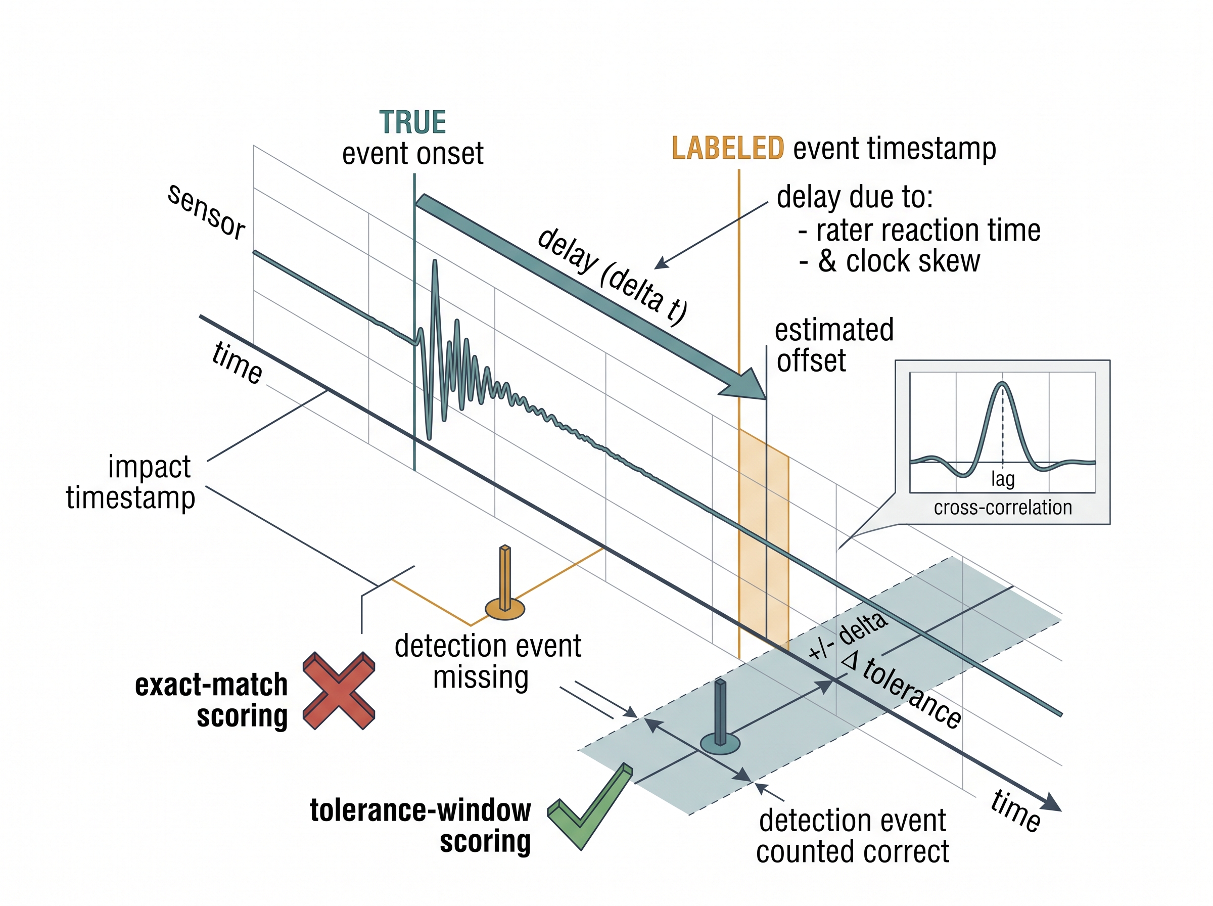
Fidelity is only one axis on which a label can fail: even a perfectly accurate label is worthless if it is pinned to the wrong instant. What. Label delay is a temporal offset between when an event happens in the signal and when its label is timestamped. Why it is endemic to sensing. Reaction time (a rater presses a marker after they notice the event), annotation-tool lag, clock skew (the two devices' clocks drifting apart over time) between the labeling device and the sensor (see synchronization in Chapter 3), and retrospective charting (a nurse logs "seizure at 14:05" from memory) all shift labels relative to the trace. A 300 ms button-press lag is trivial for detecting an hour-long sleep stage and catastrophic for detecting a 200 ms tap gesture.

How to handle it. First, estimate the offset: cross-correlate a strong signal feature (an onset energy burst) against the label edges and read off the lag. Second, correct it by shifting the labels. When the delay is variable instead, score with tolerance: count a detection as correct if it lands within a window \(\pm\delta\) of the annotation, the standard practice in event detection scoring. Third, in causal deployment, remember that the model can only label the past. A trailing-edge label therefore carries its own structural delay, which you must budget separately from annotation lag. When it bites hardest. Short-duration events and any evaluation that demands sample-exact boundaries. If you score a delayed-label dataset with zero tolerance, you will punish a correct model for the annotator's reflexes. Figure 5.6.2 illustrates label delay and temporal misalignment in event scoring.

Measuring and living with label noise

Noise, weakness, and delay all leave the same residue, a fraction of windows whose recorded label is wrong, and the closing move is to hunt those windows down. You cannot fix what you cannot find. Confident learning gives a practical, model-agnostic way to locate likely-mislabeled windows: train a classifier with cross-validation so every example gets an out-of-fold predicted probability, where out-of-fold means the prediction comes from a model that never saw that example during training, then flag examples the model confidently disagrees with. Examples where the given label has low self-confidence and another class has high confidence are your prime suspects for relabeling. The snippet below implements the core idea on a windowed sensor dataset.

Confident learning, precisely. It is a model-agnostic procedure that estimates the joint distribution between the labels on file (possibly wrong) and the true latent classes, using only a classifier's out-of-fold predicted probabilities and per-class confidence thresholds, never an external oracle. It turns the vague question "which labels are wrong?" into a calibrated ranking: count how often the model confidently prefers a class other than the recorded one, normalize those counts into an estimated noise matrix, and order windows by their probability of being mislabeled. Reach for it when you have enough data to cross-validate reliably. When the dataset is too small for trustworthy out-of-fold probabilities, prefer a robust loss or cleaner labels instead.

import numpy as np
from sklearn.ensemble import HistGradientBoostingClassifier
from sklearn.model_selection import cross_val_predict

def suspect_labels(X, y, threshold=0.5):
    """Flag windows whose given label is likely wrong.
    X: (N, D) window features; y: (N,) integer labels."""
    clf = HistGradientBoostingClassifier(max_iter=200)
    # out-of-fold probabilities: no window scores itself
    proba = cross_val_predict(clf, X, y, cv=5, method="predict_proba")
    self_conf = proba[np.arange(len(y)), y]        # P(given label)
    best_other = proba.max(axis=1)                 # P(model's pick)
    pred = proba.argmax(axis=1)
    # low confidence in the given label, high in a different class
    suspect = (pred != y) & (self_conf < threshold) & (best_other > 0.7)
    return np.where(suspect)[0], self_conf

rng = np.random.default_rng(0)
X = rng.normal(size=(2000, 16))
y = (X[:, 0] + 0.3 * rng.normal(size=2000) > 0).astype(int)
y[:40] = 1 - y[:40]                                # inject 40 flipped labels
idx, conf = suspect_labels(X, y)
print(f"flagged {len(idx)} windows; "
      f"{np.sum(idx < 40)}/40 injected errors caught")

The audit above does not silently overwrite labels; it produces a queue for a human to re-check, cheapest-first. That distinction matters: automated relabeling of your own suspects can amplify the model's biases, whereas targeting scarce annotator time at the highest-suspicion windows is almost pure upside.

What's Next

In Section 5.7, we make all of these decisions reproducible. Windowing choices, split boundaries, calibration constants, and now label provenance and label-model versions become part of a versioned data contract, so that when your labels improve or your delay estimate changes, every downstream artifact can be rebuilt and re-evaluated without guesswork.