Section 5.2: Window construction and labeling

"A sensor stream has no rows. You invent them, and then you spend the rest of the project living with the ones you chose."
A Pragmatic AI Agent

The Big Picture

Almost every model you will build in this book expects fixed-shape inputs: a tensor of $L$ timesteps by $C$ channels. But real sensors deliver an unending stream of samples with no natural row boundaries. Windowing is the act of cutting that stream into training examples, and labeling is the act of deciding what each cut means. These two choices are quietly among the most consequential decisions in a typical sensor project. They set your effective sample size, your class balance, your latency budget, and (as the next section will show) whether your test accuracy is real or an illusion. Get windowing wrong and no amount of model tuning recovers it.

This section assumes you are comfortable with sampling rate, the sampling interval $\Delta t = 1/f_s$, and timestamp alignment across channels, all covered in Chapter 3. Here we take a synchronized, uniformly sampled multichannel stream as the input and turn it into a labeled dataset that a model can consume. We stay deliberately out of the way of Section 5.3 (leakage) and Section 5.4 (splits); windowing decisions cause most leakage, so we flag the trap here and treat the cure there.

Why we cut streams into windows

Cut this wrong and every number downstream inherits the mistake: a mislabeled window teaches the model the wrong thing, and an overlapping one can inflate your reported accuracy into fiction that only collapses in the field. It is worth knowing exactly what a window is before you carve millions of them. What. A window is a contiguous slice of the stream, $x_{t:t+L}$, of fixed length $L$ samples, treated as one example. Why. Three forces demand it. Models with fixed input tensors (convolutional neural networks (CNNs), most transformers, classical feature extractors) need a fixed $L$. Labels usually apply to spans of time, not to individual samples: "walking" is a property of a two-second stretch, not of one accelerometer reading. And decisions are made on a cadence: a fall detector must emit a verdict every fraction of a second, so it must consume the stream in bites of roughly that size.

Checkpoint

So far: a window is one fixed-length slice of the stream treated as a single training example, and we cut streams into windows because models need fixed-shape inputs, labels describe spans of time rather than lone samples, and detectors must reach a verdict on a regular cadence.

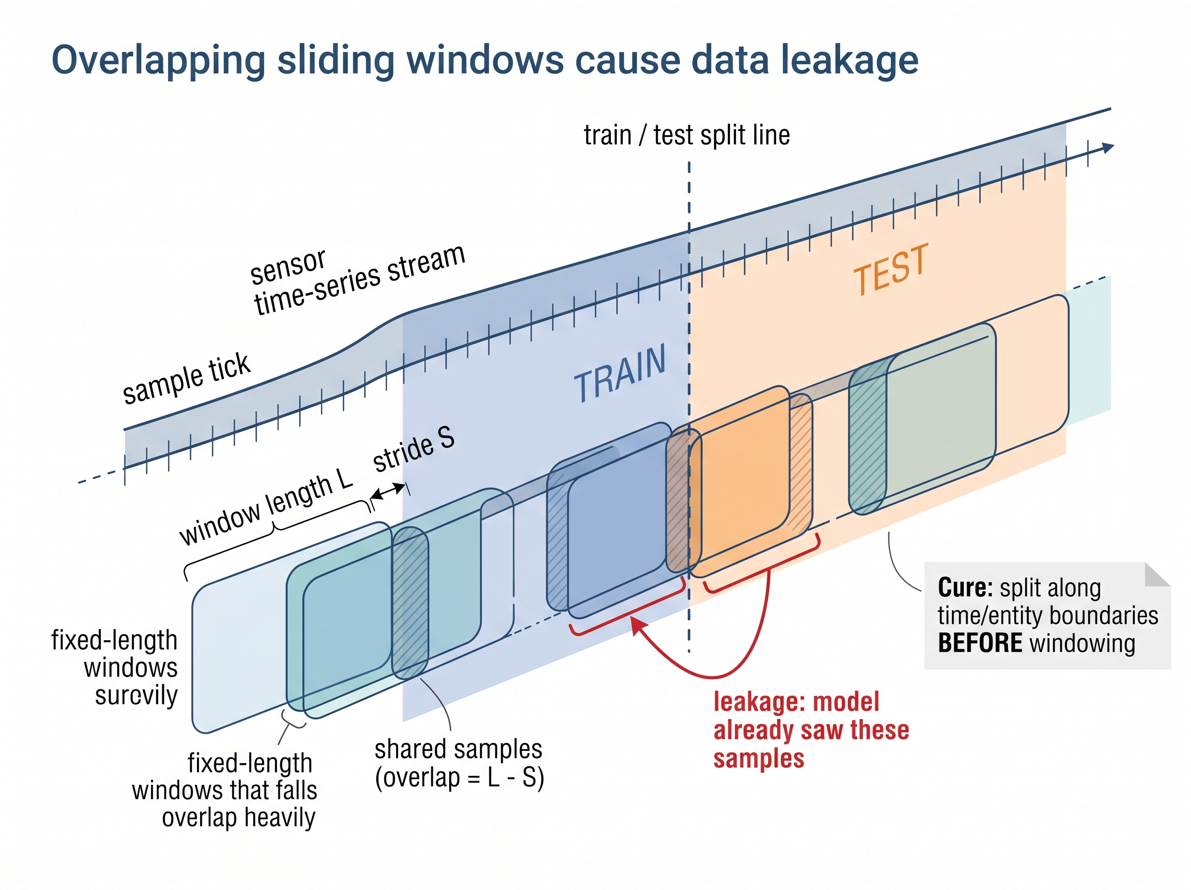
How. You choose three numbers. The window length $L$ (how much context each example holds), the stride or hop $S$ (how far you advance between consecutive windows), and the windowing policy (fixed-rate sliding, non-overlapping tumbling, or event-triggered, meaning a new window is opened only when a detected event such as a peak or threshold crossing fires). The overlap fraction follows as $1 - S/L$. When $S = L$ the windows tile the stream with no overlap (tumbling); when $S < L$ they overlap; when $S > L$ you drop samples between windows. Figure 1 shows a length-$L$ frame sliding across a raw stream by a stride $S$ smaller than $L$, so consecutive windows share the shaded overlap region.

Figure 1. A length-$L$ window sliding across a sample stream by a stride $S < L$. Windows 1, 2, and 3 each span $L$ samples but start $S$ samples apart, so adjacent windows share an overlap of $L - S$ samples (shaded). The overlap fraction is $1 - S/L$.

Stride, precisely. The stride $S$ is the number of samples the window advances between one example and the next, so it sets both how many windows a stream yields and how often a deployed model emits a fresh verdict. It matters because it is the single lever that trades dataset size and responsiveness against redundancy: every sample the stride skips is context you never score, and every sample two windows share is correlation you must account for when you split. Mechanically you slide the length-$L$ frame forward by $S$ samples and read off each frame as one example. Reach for a small stride when you want dense coverage or more training windows, and a large stride (up to $S = L$) when you want non-redundant examples or a cheaper, lower-cadence deployment. In short: a window is a decision, not a row you were handed, and the length and stride you pick quietly fix your sample size, your latency, and whether your accuracy is real.

Key Insight

Overlap is a data-augmentation knob and a leakage hazard wearing the same coat. Setting $S \ll L$ multiplies your window count and smooths class boundaries, which flatters training. But two overlapping windows share raw samples, so if one lands in train and its neighbor in test, the model has effectively seen the answer. The rule that saves you: choose overlap for the training signal you want, then split along time or entity (subject, device, or recording session) boundaries so overlapping windows never straddle the split. The augmentation is legitimate; the leakage is not, and the two are separable. Figure 5.2.1 illustrates Overlapping-window leakage across a train/test split.

Overlapping-window leakage across a train/test split — Figure 5.2.1: How heavily overlapping windows leak information across a naive train/test split: two adjacent windows share most of their samples, so when one lands in train and its near-identical neighbor in test, the model is effectively evaluated on data it has already seen, which is prevented by splitting along time or entity boundaries before windowing.

Mental Model

Picture slicing a long loaf of bread. Slide the knife only a couple of millimeters between cuts and you get many slices, but each is almost the same bread as its neighbor; slide a full slice-width and every piece is distinct. The sliding distance is your stride, and the loaf shared between two adjacent slices is the raw samples two overlapping windows share. Now imagine judging a baker with a blind taste test: if two near-identical slices go one to practice and one to the exam, the baker "passes" by having already tasted the answer. The same tiny hop that hands you more slices is what lets a practice slice leak onto the test plate, which is why the cure is to divide the loaf into train and test regions before you start sliding the knife, not after.

Choosing window length and stride

Having seen why overlap is at once a training gift and a leakage trap, we can now pin down the two numbers that govern it: the window length and the stride. What drives $L$. The window must be long enough to contain the phenomenon and short enough to stay homogeneous. Match it to the physical timescale of the signal: at least one full cycle of the slowest relevant component, and ideally a few. A human gait cycle is roughly 1 second, so 2 to 3 second windows are standard for activity recognition. A cardiac cycle is under a second; electrocardiogram (ECG) beat classifiers often window a single beat plus margin. A bearing-fault signature repeats at the shaft rotation frequency, so the window must span several revolutions to resolve it (a theme picked up in Chapter 36).

When to go short vs long. Short windows react faster and stay purer, one label each, but starve the model of context and inflate variance. Long windows are richer and more stable, yet slow to react and prone to mixing two activities. Latency versus context is a real tradeoff you design, not a default. What drives $S$. Stride sets deployment cadence and dataset size: in production the model re-runs every $S$ samples, so $S$ is a latency and compute budget, while in training a smaller stride harvests more correlated windows.

Common Misconception

The misconception is "shrinking the stride multiplies my window count, so it multiplies my effective sample size and gives the model proportionally more to learn from." It does not: windows carved from the same stretch of signal at heavy overlap are almost identical, so they carry very little independent information, and your effective sample size grows far more slowly than the raw window count while the extra near-duplicates mostly inflate optimistic evaluation when they cross a naive split.

Practical Example: a wrist wearable that keeps missing the first few seconds

A team building a smartwatch activity classifier picked 10-second windows because longer context lifted validation F1 (the F1 score, the harmonic mean of precision and recall, is a single accuracy number that stays honest under class imbalance). In the field, users complained the watch was slow to notice they had started running. The cause was structural: with a 10-second tumbling window, the model could not commit to "running" until a full 10 seconds of running had accumulated and closed a window, so the median detection delay approached 10 seconds. The fix was not a better model but a windowing change: keep the 10-second context but slide it with a 1-second stride, so a fresh verdict lands every second on a mostly-running window. Same $L$, smaller $S$, latency dropped roughly tenfold. The lesson: $L$ buys accuracy, $S$ buys responsiveness, and you tune them separately.

Real-World Application: Apple Watch fall detection

Apple Watch fall detection windows the wrist accelerometer and gyroscope stream into short overlapping frames and scores each frame for the impact-then-stillness signature of a fall. The window must be long enough to capture the arc from stumble to impact yet short enough to fire before the roughly 60-second countdown that dials emergency services, exactly the length-versus-latency tradeoff this section describes. Apple reportedly tuned the window and threshold on tens of thousands of hours of real fall and daily-activity recordings so the sliding decision fires on impacts without drowning users in false alarms.

Assigning labels to windows

Once a window is cut, what is its label? The label is unambiguous only when the entire stream carries one class. In practice a window can span a label boundary, and you need an explicit policy. The common ones:

Majority / mode. Assign the label held by the plurality of samples in the window. Simple, robust, but blurs transitions and can invent a label the user never actually held for the full window.
Center (or last) sample. Take the label at the window's midpoint or trailing edge. The trailing edge matches causal deployment, where you only know the past; the center is better for offline analysis.
Purity threshold. Keep the window only if one label covers at least a fraction $\tau$ (say 80%) of it; otherwise discard it as a transition window. This trades sample count for label cleanliness.
Dense / per-timestep. Do not collapse at all. Keep a label per sample and train a sequence-labeling model (segmentation). Richest, but demands per-sample annotations, which are expensive (see Section 5.6).

Formally, majority labeling of the window starting at $t$ is

$$ y_t = \arg\max_{c}\ \sum_{i=t}^{t+L-1} \mathbb{1}[\,\ell_i = c\,], $$

where $\ell_i$ is the per-sample annotation. Transition windows, where no class dominates, are exactly the ones this rule labels least reliably, which is why a purity threshold is often layered on top. Your labeling policy also sets class balance: discarding transition windows or collapsing a mixed span to a single label can systematically thin or thicken individual classes, so tally the post-windowing class counts rather than assuming they mirror the raw stream.

Watch Out: label delay and edge effects

Two subtle biases live at window edges. First, if annotations were recorded with a lag (a rater pressed a button a beat after the event began), your label boundaries are shifted, and short windows near transitions inherit the wrong class. Second, causal (trailing-edge) labeling means the window is labeled by its end, so an event only becomes visible once it has filled enough of the window to survive your policy. Budget for this delay explicitly rather than discovering it in the field, as the wearable team above did.

From stream to array: the mechanics

Those labeling policies, and the length-and-stride choices that precede them, only become a dataset once you express them in code, so here is the mechanical core. Concretely, windowing a synchronized array is a strided view plus a label reduction. The code below turns a $(T, C)$ stream and a length-$T$ label vector into $(N, L, C)$ windows with majority labels. It uses NumPy's zero-copy sliding-window view, so you never materialize $N$ copies of overlapping data.

import numpy as np
from numpy.lib.stride_tricks import sliding_window_view
from scipy import stats

def windowize(x, labels, L, S):
    """x: (T, C) stream; labels: (T,) per-sample labels.
    Returns windows (N, L, C) and majority label per window (N,)."""
    # sliding_window_view gives (T-L+1, C, L) views with stride 1...
    views = sliding_window_view(x, window_shape=L, axis=0)  # (T-L+1, C, L)
    views = views.transpose(0, 2, 1)                        # (T-L+1, L, C)
    starts = np.arange(0, len(views), S)                    # apply the hop
    windows = views[starts]                                 # (N, L, C)

    lbl_views = sliding_window_view(labels, L)[starts]      # (N, L)
    y = stats.mode(lbl_views, axis=1, keepdims=False).mode  # majority vote
    return windows, y

# 3 s windows, 1 s hop on a 50 Hz stream: L=150, S=50
X = np.random.randn(10_000, 6)              # 200 s of 6-axis inertial measurement unit (IMU) at 50 Hz
lab = np.repeat([0, 1, 2, 1], 2500)         # 4 activity blocks
W, y = windowize(X, lab, L=150, S=50)
print(W.shape, y.shape)                     # (198, 150, 6) (198,)

Zero-copy sliding-window construction with majority labeling. sliding_window_view avoids copying overlapping samples until you index starts, so memory stays flat even at heavy overlap; the stats.mode reduction implements the majority policy from the previous section.

The snippet above is deliberately explicit so the mechanics are visible: strided view, hop selection, label reduction. In a real pipeline you rarely write it by hand.

Step-Through: majority windowing on an 8-sample stream

Trace windowize with a tiny example so every index is concrete. Take a stream of $T = 8$ samples with one channel, per-sample labels $\ell = [0,0,0,1,1,1,1,1]$, window length $L = 3$, and stride $S = 2$. Step 1, the sliding view produces $T - L + 1 = 6$ candidate windows starting at samples 0, 1, 2, 3, 4, 5. Step 2, the hop selects starts = [0, 2, 4], giving $N = 3$ windows. Step 3, read off and vote each one: window at start 0 covers samples 0 to 2 with labels $[0,0,0]$, so the majority is 0; window at start 2 covers samples 2 to 4 with labels $[0,1,1]$, so the majority is 1; window at start 4 covers samples 4 to 6 with labels $[1,1,1]$, so the majority is 1. Result: W.shape == (3, 3, 1) and y == [0, 1, 1]. Notice the middle window straddles the 0 to 1 transition and gets labeled 1 by a 2-to-1 vote; a purity threshold of $\tau = 0.8$ would discard it, because no single label covers 80% of its three samples.

Right Tool: let a windowing library carry the bookkeeping

Purity thresholds, per-window timestamps, dropping partial trailing windows, and grouping by recording so windows never cross session boundaries add up to roughly 40 to 60 lines of fiddly, bug-prone code. Libraries such as tsfresh's roll utilities, sktime's sliding-window transformers, or a few lines of pandas DataFrame.rolling plus groupby collapse that to about 3 to 5 lines and, critically, keep windows inside their group so you do not accidentally splice two devices together. You still choose $L$, $S$, and the label policy; the library just stops the off-by-one and cross-boundary bugs. Section 5.4 treats these group-aware splits, and why crossing a group boundary corrupts evaluation, in full.

The window that outran the phoneme

The 25-millisecond frame with a 10-millisecond hop is so standard in speech recognition that it feels like a law of physics, but it is really an artifact of 1960s tape and tube hardware. Engineers picked roughly 25 ms because that is about the longest a speech signal stays quasi-stationary (short enough that the vocal tract has not reshaped, long enough to resolve pitch), and 10 ms simply because it gave a convenient 100 frames per second on the clocks of the day. Two human generations and several deep-learning revolutions later, the log-mel and mel-frequency cepstral coefficient (MFCC) frontends that still feed most speech pipelines slide that same 25/10 window (self-supervised raw-waveform models such as wav2vec 2.0 instead learn features on a roughly 20-millisecond frame stride), making the 25/10 frame one of the oldest surviving hyperparameters in machine perception, chosen for a physiological timescale that has not changed since we started measuring it.

Research Frontier

A 2023 line of work questions the hand-chosen fixed window itself. PatchTST (Nie et al., ICLR 2023, "A Time Series is Worth 64 Words") slices a series into patches and lets a transformer attend across them, showing that patch length behaves like a learnable representational choice rather than a fixed preprocessing constant; time-series foundation models such as MOMENT (Goswami et al., ICML 2024) and Moirai (Woo et al., 2024) push this further by pretraining on masked patches so a single model transfers across sensing tasks with minimal per-task window tuning. The direction to watch: the patch or window becomes a pretrained, transferable unit instead of a project-specific hyperparameter, though $L$ and $S$ still bound latency, cadence, and leakage exactly as this section describes.

Exercise

Take a labeled 50 Hz IMU recording with four activity blocks. (a) Window it at $L = 150$ with strides $S \in \{150, 75, 15\}$ and report how many windows each produces and what fraction are "transition" windows (no label covering 80%). (b) Add a purity filter at $\tau = 0.8$ and recount. (c) Explain in two sentences why the $S = 15$ dataset will make a random train/test split look far more accurate than it truly is, and how you would split instead. Verify your reasoning against Section 5.3.

Self-Check

You need a fall detector to respond within 0.5 s but a fall signature spans 2 s. Which knob do you change, $L$ or $S$, and why can you not simply shrink $L$ to 0.5 s?
Your dataset has 90% overlap between adjacent windows. Name one training benefit and one evaluation danger of that choice.
Under trailing-edge (causal) labeling, why does a freshly started activity take a while to appear in the labels even with a small stride?

Try It: measure the overlap-leakage gap yourself

With a laptop, NumPy, and scikit-learn you can watch overlap manufacture fake accuracy in about twenty lines:

Synthesize a labeled 50 Hz stream: X = np.random.randn(10_000, 6) and lab = np.repeat([0, 1, 2, 1], 2500), then reuse the windowize(X, lab, L, S) function from earlier in this section.
Build two datasets from the same stream: a non-overlapping one with S = 150 and a heavily overlapping one with S = 15 (90% overlap). Flatten each window to a vector with W.reshape(len(W), -1).
For each dataset, run a naive random split (sklearn.model_selection.train_test_split, 80/20, shuffle on) and train a RandomForestClassifier; record the test accuracy.
Now split the same two datasets by time instead: put the first 80% of windows in train and the last 20% in test (no shuffle), retrain, and record accuracy again.
Line up the four numbers. The random split on S = 15 should look the strongest and should fall the most when you switch to the time split; that drop is exactly the leakage the overlap created, and it is invisible until you split correctly.

Lab: sweep the stride and watch the tradeoffs move

Goal. In 15 to 30 minutes, feel window length and stride change three quantities at once: window count, transition-window fraction, and apparent accuracy under a naive split.

Tools. Python with NumPy, scikit-learn, and matplotlib. Use the public UCI HAR dataset (30 subjects, 50 Hz smartphone IMU) or synthesize a labeled stream with X = np.random.randn(20_000, 6) and lab = np.repeat([0,1,2,3,1,0], ...). Reuse the windowize(X, lab, L, S) function from this section.

What to vary. Fix $L = 128$ and sweep the stride $S \in \{128, 64, 32, 16, 8\}$ (overlap 0% up to about 94%). At each setting also toggle a purity filter at $\tau = 0.8$ on and off.

What to observe. For each $S$ plot (1) the number of windows, (2) the fraction dropped as transition windows by the purity filter, and (3) two test accuracies from a RandomForestClassifier on flattened windows: one from a shuffled 80/20 split and one from a time-ordered split (first 80% train, last 20% test). Watch the shuffled-split accuracy climb as $S$ shrinks while the time-split accuracy stays flat or falls; the widening gap between the two curves is leakage you manufactured purely by overlapping windows, and it is the empirical preview of Section 5.3.

Windowing and labeling turn a formless stream into rows you can model, evaluate, and split. Those rows are the atoms of everything downstream, from feature extraction to human activity recognition to leakage-safe benchmarking in Chapter 65. The choices here propagate through the whole project, so decide them on purpose, write them down, and version them with the pipeline.

What's Next

In Section 5.3, we confront the field's most common and most expensive error: leakage. We will see exactly how overlapping windows, shared subjects, and normalization computed on the full dataset let information from the test set bleed into training, why the resulting accuracy numbers are fiction, and the concrete disciplines that keep your evaluation honest.