Leakage in sensor datasets (the field's most common error)

"The model did not learn the task. It learned who was holding the sensor, and I paid it a 99% accuracy for the trouble."

A Chastened AI Agent

This section builds directly on Section 5.2, where we cut streams into overlapping windows, and it assumes you understand autocorrelation and the sampling model from Chapter 3. It also foreshadows Chapter 65, which turns these ideas into full evaluation protocols. We stay out of the mechanics of building splits (that is Section 5.4) and of normalization (Section 5.5); our job is to define leakage precisely and make it visible.

What leakage is, formally

What. Train a model on \(\mathcal{D}_{\text{train}}\) and evaluate it on \(\mathcal{D}_{\text{test}}\). Leakage is any dependency that biases the test estimate of generalization error toward optimism. The measured performance then overstates what the model will achieve on genuinely unseen data from the deployment distribution. Why it matters. A held-out test set exists to stand in for the future. If the test set shares information with training that the future will not share, the stand-in lies, and every decision that rests on it (model selection, go/no-go, a regulatory claim) rests on fiction. How it shows up. An honest evaluation requires that the train and test examples be independent given the label, so that

Leakage breaks the independence. The split shares some latent variable \(z\) (a subject's physiology, a device's calibration offset, a moment in time), so the model exploits \(z\) to answer test queries it should not be able to answer. On tabular data you can often arrange this independence easily. On sensor data, violating it is the default, which is why leakage is endemic here.

Concretely, a held-out test set is a partition of the labeled data that is quarantined before any training, tuning, or feature choice touches it, and is scored exactly once to produce an estimate of deployment error. It matters because it is the only unbiased instrument you have for the future: the instant it influences a modeling decision it stops measuring generalization and starts measuring memorization. Mechanically it works by simulating the train-then-deploy gap, standing in for data the model has never encountered; reach for it when you need an honest point estimate, and prefer nested cross-validation instead when data is too scarce to spend a whole partition on a single measurement. In short: a sensor test set tells the truth only when no identity it has already seen is allowed to answer for the future.

A field guide to the leaks

Leakage in sensor pipelines is not one bug but a family. Learn to recognize each by where it enters. Figure 5.3.2 illustrates the five doors of leakage in a sensor ML pipeline.

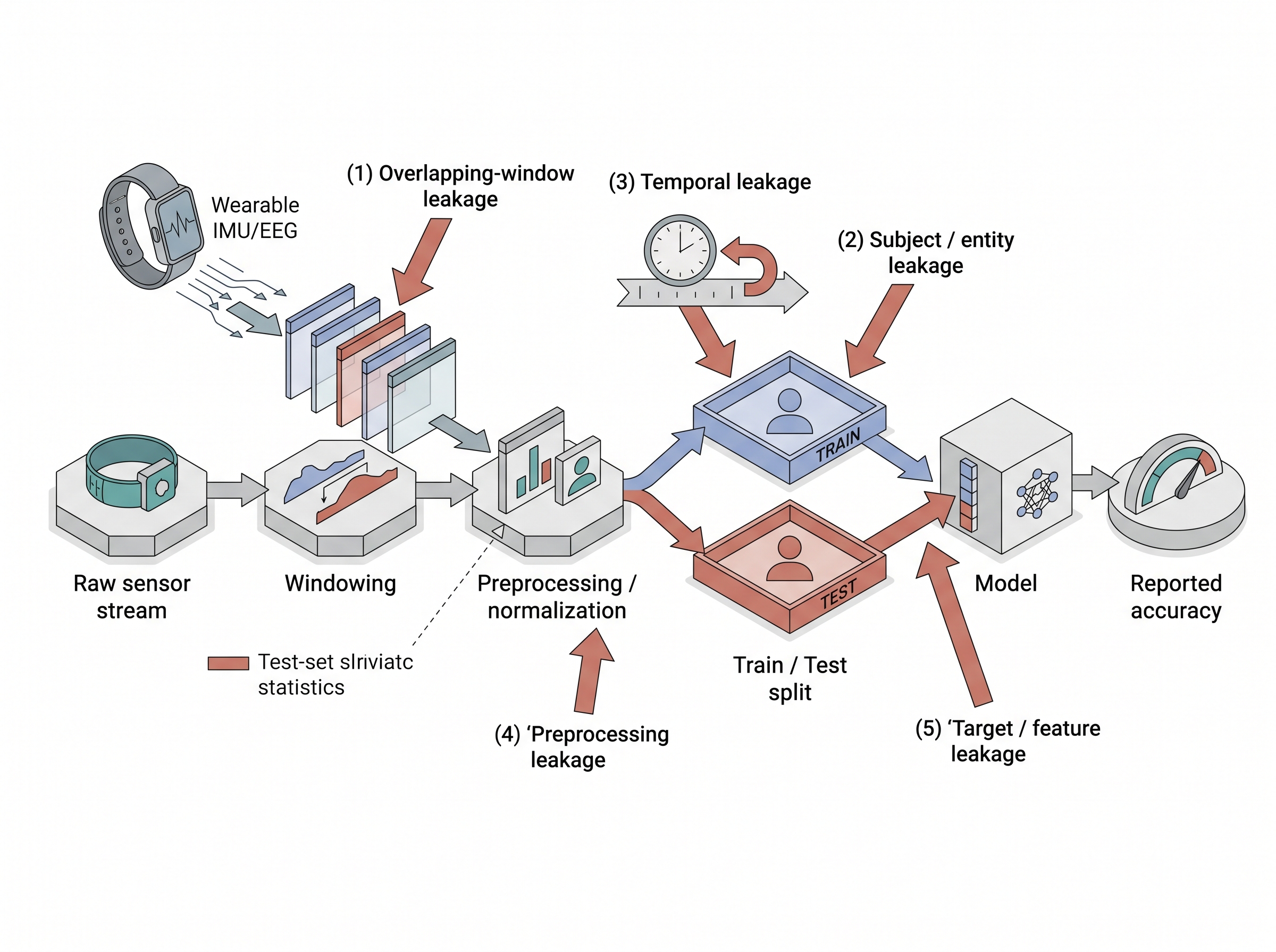
• Overlapping-window leakage. Adjacent windows from a sliding stride share raw samples (Section 5.2). Split the windows at random and near-duplicate neighbors land on opposite sides; the test window is a lightly shifted copy of a training window. This alone can add tens of points of phantom accuracy.
• Subject / entity leakage. The same person, patient, vehicle, or machine appears in both train and test. The model recognizes the entity's signature and rides its label correlation. This is the dominant leak in human activity recognition, biosignals, and predictive maintenance.
• Temporal leakage. Training on data recorded after the test period, or shuffling a non-stationary stream (one whose statistical properties, such as mean or variance, drift over time) so the future informs the past. Any deployed system only ever sees the past, so a random shuffle over time is a lie about causality.
• Preprocessing leakage. Computing normalization statistics, principal component analysis (PCA) bases, resampling filters, or feature scalers on the full dataset before splitting, so test-set statistics flow into the training transform. Subtle, common, and fully preventable by fitting transforms on train only (Section 5.5).
• Target / feature leakage. A feature encodes the label by construction: a maintenance log field that is only populated after a failure, a filename that contains the class, a sensor that was added specifically because a fault was already known. The model reads the answer off the input.

Seeing the leak: the accuracy gap

A published 0.98 that collapses to 0.71 in the clinic is not a rounding error; it is a recalled device, a retracted paper, or a safety review, each one tracing back to a number nobody stress-tested. Before you trust any headline score you need a way to measure how much of it is real. Naming a leak tells you where to look; the accuracy gap tells you how much it is costing you. How to detect it. The most reliable diagnostic is a controlled comparison: evaluate the identical model and features under a naive random split and under an entity-disjoint split (one where no subject, device, or session appears on both sides, built as shown in Section 5.4), and read the gap. A large drop is the leakage magnitude. The code below builds a tiny synthetic dataset where each subject has a strong personal offset that is predictive within a subject but useless across subjects, then measures both numbers. Figure 5.3.1 contrasts the two splitting strategies: the random split scatters each subject's windows across both partitions, while the subject-disjoint split keeps every subject wholly on one side.

import numpy as np
from sklearn.ensemble import RandomForestClassifier
from sklearn.model_selection import train_test_split, GroupShuffleSplit

rng = np.random.default_rng(0)
n_subj, per_subj = 20, 200
# Each subject gets a private fingerprint offset; the TRUE label depends
# only on a within-window feature, not on the offset.
subj = np.repeat(np.arange(n_subj), per_subj)
fingerprint = rng.normal(0, 3, n_subj)[subj]          # identity nuisance
signal = rng.normal(0, 1, len(subj))                  # the real, learnable cue
y = (signal > 0).astype(int)
X = np.c_[signal + fingerprint, fingerprint + rng.normal(0, .1, len(subj))]

# (1) Naive random split: subjects appear on both sides -> leakage
Xtr, Xte, ytr, yte = train_test_split(X, y, test_size=.3, random_state=0)
leaky = RandomForestClassifier(random_state=0).fit(Xtr, ytr).score(Xte, yte)

# (2) Subject-disjoint split: no subject crosses the boundary
gtr, gte = next(GroupShuffleSplit(test_size=.3, random_state=0).split(X, y, subj))
honest = RandomForestClassifier(random_state=0).fit(X[gtr], y[gtr]).score(X[gte], y[gte])

print(f"random split:  {leaky:.3f}")   # optimistic, leaks identity
print(f"group split:   {honest:.3f}")  # what deployment actually sees

Run it and the random-split score sits well above the group-split score, because that evaluation let the forest read the identity offset it also saw in training. The group split forces reliance on signal, the only cue that transfers to a new subject, and the gap between the two is what leakage costs you. Three cheap reflexes catch most leaks: shuffle-test a suspiciously strong feature (if performance survives label shuffling, it is leaking), inspect what the model attends to (identity artifacts light up), and ask whether each feature would be knowable at prediction time in production.

Leakage is not an exotic failure; it is the default outcome of treating an autocorrelated, identity-tagged sensor stream like a bag of independent rows. The habit that protects you is to name, before any model runs, the entity that must never cross the split and the moment in time that separates past from future, then to enforce both mechanically. Do that and your test set goes back to doing its one job: telling you the truth. The same discipline reappears everywhere models are evaluated in this book, from patient-level biosignal splits to leakage-safe benchmarking in Chapter 65.

What's Next

Section 5.4 turns the diagnosis into a cure: how to construct device, user, site, session, and machine splits that hold the leakage boundary you identified here. It shows when each grouping key is the right one, how to keep class balance across disjoint groups, and how to layer grouping with time-based splits so both identity and causality are respected at once.