Transfer functions and response time

"By the time I finish reporting the temperature, the temperature has moved on. I spend my whole life describing a world that no longer exists."

A Perpetually Late AI Agent

Static and dynamic transfer functions are two different questions

The word transfer function is overloaded, and separating its two meanings is the first job. The static transfer function is the input-output relationship after everything has settled: hold the stimulus fixed, wait, and record the reading. This is the calibration curve from Section 2.2, ideally the straight line \(y = k\,x + b\) with sensitivity \(k\) and offset \(b\). It answers where the reading lands. It says nothing about when.

The dynamic transfer function answers the "when." It describes how the output evolves in time when the input changes, and it exists because every sensor stores energy somewhere: heat in a thermal mass, charge on a capacitance, momentum in a proof mass (the small internal test mass whose motion an accelerometer measures). That storage cannot change instantly, so the output cannot either. Why does this deserve its own section rather than a footnote? Because for any signal that moves, the dynamic behavior typically dominates the error budget. A thermometer with a perfect calibration curve is still useless for catching a two-second temperature spike if it takes thirty seconds to respond. The static curve is a portrait; the dynamic transfer function is the sensor caught mid-stride. In short: calibration tells you where a sensor lands, but only its transfer function tells you whether you can trust it before then.

The first-order model and its time constant

Misjudge a sensor's dynamics and every decision built on its readings inherits the error: a furnace overshoots and scorches the boards, an airbag fires a beat late, a model trains on peaks the sensor never actually captured. Getting this one model right is what keeps the rest of the pipeline honest. To turn that mid-stride portrait into numbers you can actually predict, we need a model of the dynamics, and one remarkably simple model covers the vast majority of real devices. The overwhelming majority of sensors, at least to first approximation, behave as first-order linear systems. One number, the time constant \(\tau\), captures their entire dynamic personality. The governing rule is intuitive: the output chases the input, and its rate of catch-up is proportional to how far behind it is. Writing \(y(t)\) for the reading and \(u(t)\) for the true stimulus,

Precisely, the time constant is the ratio of a system's stored-energy capacity to its rate of exchange with the outside world (for a thermal probe, its heat capacity divided by its thermal conductance), and it carries units of seconds. It matters because it is the single number that turns a sensor's physical construction into a quantitative promise about speed, letting you predict lag before you ever apply a signal. Mechanistically it sets how quickly the output can relax toward the input: a larger \(\tau\) means more stored energy to shuffle and therefore a lazier response. Reach for this one-parameter first-order model whenever a sensor has one dominant energy store and no springiness, and switch to the two-parameter second-order model later in this section once mass and a restoring force let the response overshoot and ring.

The step response

Now subject it to the experiment engineers actually run, a step input: at \(t = 0\) plunge the sensor from a value it had settled at into a new constant stimulus. The solution is the exponential approach every practitioner should have memorized,

where \(y_0\) is the starting reading and \(y_\infty\) the final one. The time constant \(\tau\) is the moment the sensor has closed \(1 - e^{-1} \approx 63.2\%\) of the gap. After \(3\tau\) it has covered \(95\%\), the common "settled" criterion; after \(5\tau\), \(99.3\%\), the stricter "fully settled" mark quoted for high-precision work. That single parameter also fixes the derived timings vendors like to advertise: the rise time from 10% to 90% of the step is \(t_{10\text{-}90} = \tau \ln 9 \approx 2.2\,\tau\). Figure 2.5.1 plots this exponential approach and marks the milestone crossings so you can read the whole schedule at a glance.

How do you find \(\tau\) for a sensor you hold in your hand? You do not need a lab. Apply a step, log the response, and fit the exponential. The code below simulates a first-order thermal sensor with \(\tau = 4\) seconds, then recovers that value from the noisy trace, exactly the round trip you would perform on real hardware.

import numpy as np
from scipy.optimize import curve_fit

tau_true = 4.0                      # seconds; unknown in real life
t = np.arange(0, 25, 0.1)
step = 100.0 * (1 - np.exp(-t / tau_true))          # 0 -> 100 degree step
noisy = step + np.random.normal(0, 1.5, t.size)     # add sensor noise

model = lambda t, tau, y_inf: y_inf * (1 - np.exp(-t / tau))
(tau_hat, y_inf_hat), _ = curve_fit(model, t, noisy, p0=[1.0, 90.0])

print(f"recovered tau = {tau_hat:.2f} s  (true 4.00)")
print(f"rise time 10-90% = {tau_hat * np.log(9):.2f} s")

As Listing 2.5.1 shows, characterizing a sensor's speed is a two-line fit once you have a clean step. The harder part is arranging a genuinely instantaneous step in the physical world, which is often the real experimental challenge.

Frequency response: bandwidth is response time in disguise

Step response tells you how a sensor reacts to a sudden jump. But many real signals oscillate: a vibrating bearing, a beating heart, a swaying bridge. For these, the more natural description is the frequency response, and it turns out to be the same information wearing different clothes. Feed a first-order sensor a sinusoid, and it faithfully reproduces slow oscillations but progressively attenuates (shrinks the amplitude of) and delays fast ones. The dividing line is the cutoff frequency, tied directly to the time constant:

At \(f_c\), the sensor's output amplitude has dropped to \(1/\sqrt{2} \approx 0.707\) of the true amplitude, the famous -3 dB point, and the signal lags by 45 degrees. Above it, response falls off further; the sensor cannot see fast wiggles. This is why a slow sensor and a low-bandwidth sensor are the same object. Our reflow thermocouple with \(\tau = 6\) s has a cutoff of only \(f_c \approx 0.027\) Hz, so it stays blind to anything faster than a slow half-minute swell. The reciprocal relationship \(f_c \tau\) being fixed is one of the most useful sanity checks in sensing: quote either the time constant or the bandwidth, and you have implicitly quoted the other.

This connects forward to two later ideas. Bandwidth sets the maximum meaningful sample rate: sampling a \(0.027\) Hz sensor at 1 kHz just records the same slow curve a thousand times over, a waste Chapter 3 makes precise through the Nyquist limit. And a sensor is a low-pass filter you did not choose, so reading it as one bridges to the filters you do choose in Chapter 6.

from scipy.signal import TransferFunction, lsim
import numpy as np

tau = 4.0
sensor = TransferFunction([1], [tau, 1])     # first-order low-pass, gain 1
t = np.arange(0, 25, 0.1)
u = (t > 2).astype(float)                     # a step at t = 2 s
t_out, y, _ = lsim(sensor, U=u, T=t)         # sensor's response to u

When one time constant is not enough: overshoot and latency

Everything up to here has ridden on a single time constant setting one stored-energy relaxation, but adding one more physical ingredient breaks that tidy one-number picture. Not every sensor settles politely. Add mass and a restoring spring, as in an accelerometer or a pressure diaphragm, and you get a second-order system that can overshoot: swing past the true value, ring, and settle only after a few oscillations. Its behavior is governed by two numbers, a natural frequency \(\omega_n\) (the rate at which it would oscillate if nudged and left undamped) and a damping ratio \(\zeta\). When \(\zeta < 1\) the sensor is underdamped and rings; a lightly damped microelectromechanical systems (MEMS) accelerometer near its resonance can report a transient spike far larger than the real acceleration, which a naive threshold detector will happily flag as an impact. Sensor designers usually target \(\zeta \approx 0.7\), the sweet spot that reaches the final value fastest without appreciable overshoot.

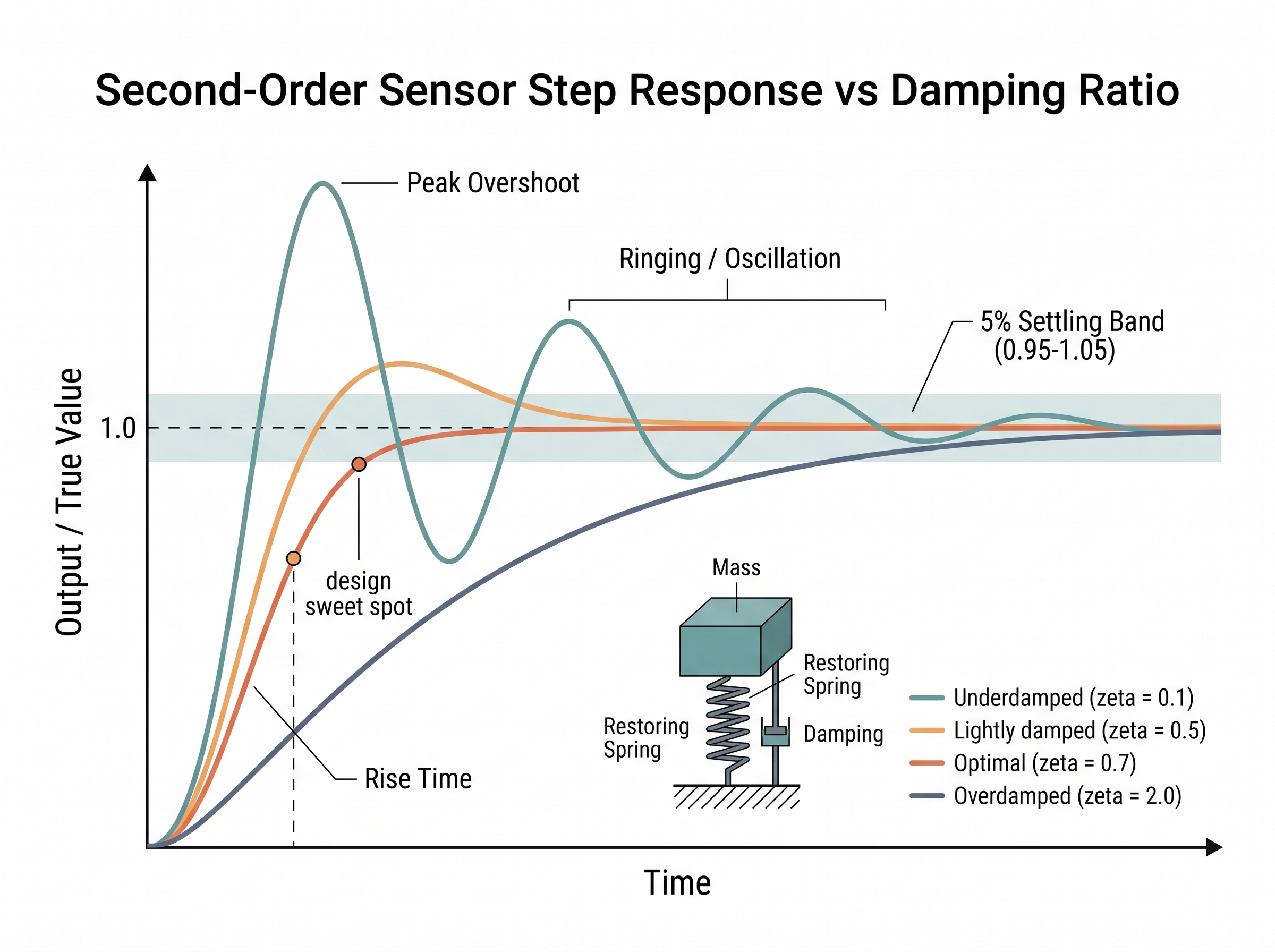
Separate from this smearing is pure latency, a fixed transport delay from processing, wireless transmission, or digital filtering inside the sensor package. Smoothing and lag are different sins: smoothing blurs a change, latency shifts it wholesale in time. Both matter enormously for anything in a control loop. Tell an estimator such as the Kalman filter in Chapter 9 a sensor's time constant and delay, and it compensates for them. It effectively runs the transfer function backward to recover a sharper estimate of the true state. But it can only undo lag it knows about, which is the entire reason this section insists you measure \(\tau\) and the delay before you trust the number.

Response time, in the end, is where the tidy static picture of Sections 2.2 through 2.4 collides with a moving world. A sensor is not a snapshot device; it is a filter with memory, and the transfer function is the exact contract stating how much of the present it will let through and how much of the past it is still reporting. Read that contract before you build on the numbers.

What's Next

Section 2.6 confronts the fact that a sensor's transfer function is rarely a function of one input alone. A humidity sensor drifts with temperature; a gas sensor responds to the wrong gas; a strain gauge answers to heat as readily as to force. That unwanted coupling, cross-sensitivity, is the next crack in the clean measurement model, and learning to model it is the last step before we assemble the full sensor equation that bridges physics to AI.