Section 2.6: Cross-sensitivity and environmental coupling

"I was hired to measure carbon dioxide. Nobody told me I would spend most of my career reporting the temperature and the weather instead."
A Disillusioned AI Agent

The big picture

A datasheet promises that a sensor responds to one thing. Physics disagrees. The same transduction that couples the sensing element to your target quantity also couples it, more weakly, to a crowd of others: temperature, humidity, supply voltage, mechanical strain, stray light, magnetic fields, aging chemistry. This section is about those unwanted couplings. Cross-sensitivity is a sensor responding to a physical quantity other than its intended measurand. Environmental coupling is the broader fact that the operating environment leaks into every reading. Ignore it and your beautiful model learns the weather instead of the phenomenon. Model it and you unlock the single most reliable accuracy win available in sensor AI: compensation. The earlier sections gave you clean, single-input pathologies (Section 2.4's bias and drift, Section 2.5's transfer function). This section is where a real sensor stops being a function of one variable and becomes a function of its whole world.

This section assumes you are comfortable with the transfer function and response time from Section 2.5, and with bias, drift, and saturation from Section 2.4. Cross-sensitivity is what turns those scalar defects into a coupled, multivariable problem. If you need the probability machinery to reason about the resulting error, Chapter 4 supplies estimation and uncertainty propagation, and the confounding structure here reappears as a leakage hazard in Chapter 5.

The coupled measurement model

Extend the single-input transfer function of Section 2.5 into a multivariable one. Let $x$ be the intended measurand and let $\mathbf{c} = (c_1, \dots, c_m)$ be the interfering environmental quantities: temperature $T$, relative humidity $RH$, supply voltage, and so on. The raw reading is

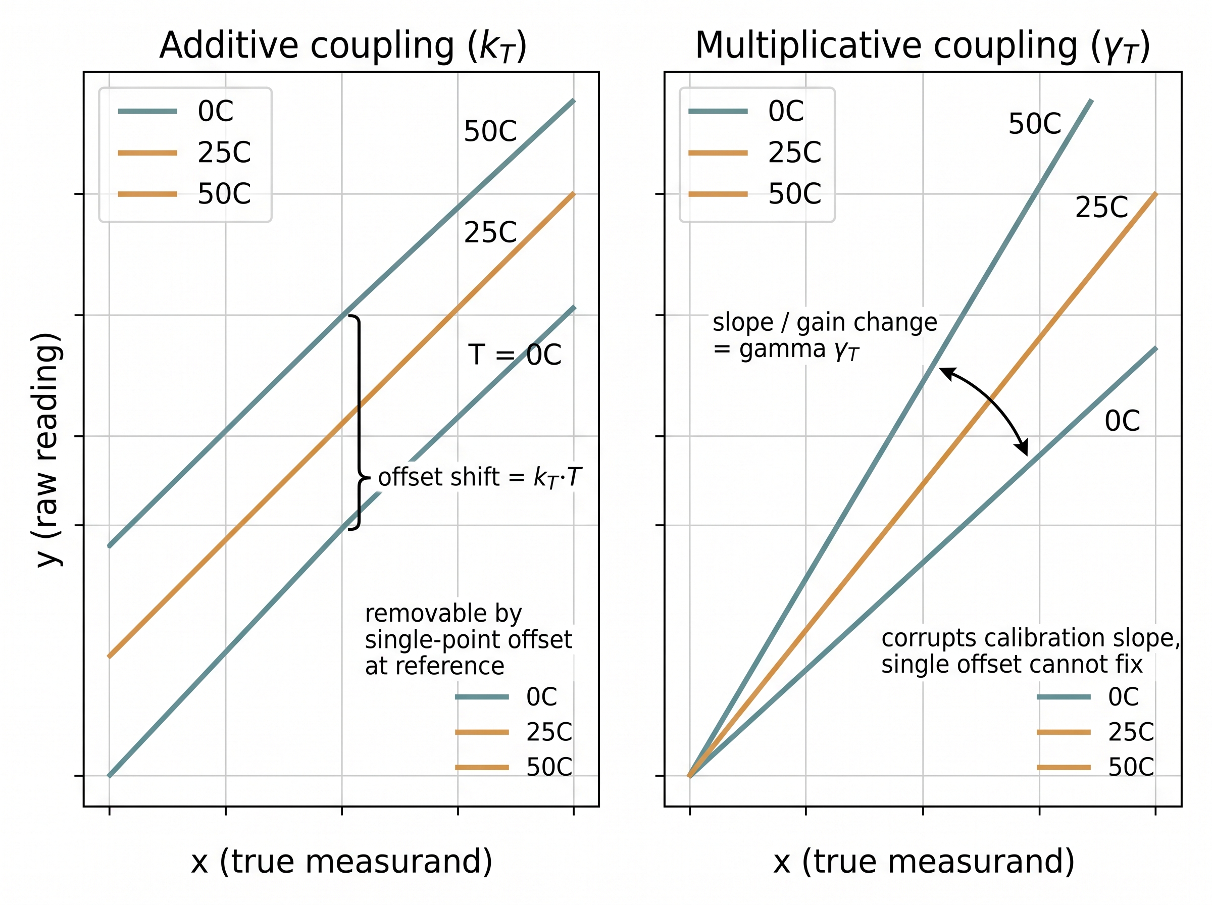
$$y = f(x, \mathbf{c}) + \varepsilon = \underbrace{S\,x}_{\text{intended}} + \underbrace{\sum_{j=1}^{m} k_j\, c_j}_{\text{cross terms}} + \underbrace{\sum_{j} \gamma_j\, x\, c_j}_{\text{gain coupling}} + \varepsilon,$$

where $S$ is the nominal sensitivity, the $k_j$ are additive cross-sensitivity coefficients (an interferer shifts the reading regardless of $x$), and the $\gamma_j$ are multiplicative couplings (an interferer scales your response to $x$). The distinction matters. An additive term looks like a drifting bias you can null out at a known reference. A multiplicative term corrupts your calibration slope, and a single-point offset cannot remove it. Temperature is the universal offender because it enters through nearly every physical mechanism: carrier mobility in silicon, resistance of metal traces, elastic modulus of a diaphragm, reaction rate of a gas-sensitive film. When a datasheet quotes a "temperature coefficient of offset" and a separate "temperature coefficient of sensitivity", it is handing you $k_T$ and $\gamma_T$ directly. In short: a sensor never measures one thing alone, so name what else it feels and you can subtract the world back out. Figure 2.6.2 illustrates additive versus multiplicative cross-sensitivity in the transfer function.

Additive versus multiplicative cross-sensitivity in the transfer function — Figure 2.6.2: Additive cross-sensitivity shifts the transfer-function intercept (parallel lines, removable at a single reference point), while multiplicative coupling rotates its slope (a fan through the origin, corrupting the calibration gain).

Key insight

Cross-sensitivity is not noise. Noise is zero-mean and averages away with more samples (Section 2.3); a cross term is a deterministic, structured function of a measurable variable. That is bad news and good news. Bad, because no amount of averaging removes it, so it survives into your features and your model. Good, because it is predictable: if you also measure the interferer, you can subtract its contribution. Most credible environmental sensors ship with an on-die temperature sensor for exactly this reason. The interferer is your best compensation feature, not just your enemy.

Where couplings come from, mechanism by mechanism

Naming the mechanism tells you which interferer to instrument and whether the coupling is additive or multiplicative. A capacitive humidity sensor measures the dielectric change of a polymer film. That same film swells with temperature, so it carries a strong $k_T$. Worse, the quantity of interest, water partial pressure, is itself temperature-dependent, which is why cheap hygrometers disagree across a warm room. A microelectromechanical systems (MEMS) accelerometer's proof mass sits on silicon springs whose stiffness drifts with temperature, so it shows both an offset shift and a sensitivity change. The same mass responds to any acceleration including gravity, so tilt cross-couples into linear-acceleration estimates (the problem Chapter 24 spends whole algorithms untangling). Electrochemical gas sensors are notoriously promiscuous: a sensor sold for carbon monoxide will happily oxidize hydrogen and other reducing gases, reporting them as CO.

Checkpoint

So far: every coupling named here traces back to a shared physical pathway between an interferer and the transducer (a swelling film, a temperature-dependent spring, a nonselective reaction), and that pathway is what tells you which channel to instrument and whether the resulting term is additive or multiplicative.

Strain gauges pick up temperature as apparent strain; optical sensors pick up ambient light; magnetometers pick up the phone's own speaker magnet and the steel in a passing elevator. The lesson is uniform: identify the shared physical pathway between the interferer and the transducer, and the coupling term follows. And once that pathway is named, the interferer stops being a mystery and becomes a quantity you can measure and subtract, which is exactly the remedy the next section builds.

Practical example: the "heart rate that tracked the sunset"

A wearables team shipping a wrist photoplethysmography (PPG) optical heart rate (HR) monitor found their overnight resting-HR estimates drifting upward by six to ten beats per minute in the last hour before dawn, on many users, indoors, at rest. No physiological cause fit. The culprit was cross-sensitivity to skin temperature and to ambient infrared: as the room cooled toward morning, peripheral vasoconstriction changed the optical path and the photodiode's dark current, the small current it produces even with no light falling on it, shifted with its own falling temperature, biasing the pulse-amplitude features the HR algorithm relied on. The fix was not a better neural network. It was adding the already-present skin-temperature channel as an input and fitting a compensation term, which collapsed the artifact and, as a bonus, improved motion robustness because temperature correlated with the user being under a blanket. The optical physics behind this coupling is the subject of Chapter 30; here the point is that the environment, not the biology, moved the number.

Real-World Application: barometric altitude in Apple and Android phones

Consumer barometers such as the Bosch BMP390 in modern phones and watches sense pressure through a piezoresistive (its electrical resistance changes as the diaphragm flexes under pressure) MEMS diaphragm whose output has a large, well-characterized temperature cross-sensitivity, so the die integrates a temperature sensor and applies factory-fit compensation coefficients before reporting pressure. Apple's CoreMotion and Android's Sensor.TYPE_PRESSURE pipelines lean on this compensated output to estimate floor-level altitude changes for indoor navigation and fall detection. Without the on-die temperature correction the reported altitude would wander by tens of meters as the phone warms in a pocket, which is exactly the additive-plus-multiplicative coupling this section models.

Compensation: measure the interferer, subtract its effect

A miscompensated sensor does not fail loudly; it ships a plausible wrong number that a downstream model then faithfully learns, which is how a heart-rate monitor tracks the sunset and a gas array alarms on a cold front. The remedy is almost embarrassingly cheap. The workhorse remedy is compensation: instrument the dominant interferers, fit the coupling coefficients on characterization data, and correct each reading. Given the additive-plus-multiplicative model above and co-recorded $T$ and other $c_j$, you recover $x$ by inverting the coupling. When temperature dominates and the interaction is mild, a low-order polynomial in $T$ captures both the offset and slope drift; fit it once per device, since coefficients vary unit to unit. The code below fits a first-order temperature compensation and reports the error reduction.

Concretely, compensation is a correction function that takes the raw reading plus the measured interferers and returns an estimate of the true measurand with the modeled cross terms subtracted back out; it matters because it converts a structured, non-averaging error into a residual that is often an order of magnitude smaller. It works by fitting the coupling coefficients (the $k_j$ and $\gamma_j$) on labeled characterization data where the interferer was deliberately varied, then algebraically inverting that fitted relationship at run time. Reach for compensation when the interferer is measurable and the coupling is stable and low-order; prefer the hardware and learned remedies later in this section when the interferer is unmeasured, the coupling drifts with age, or it turns sharply nonlinear outside the characterized envelope. Figure 2.6.1 traces this data flow: the raw reading and the measured interferers both feed a compensation function whose behavior is set by the fitted coefficients, and it returns the corrected estimate.

Figure 2.6.1: The compensation data flow. The sensor element supplies the raw reading y and the interferer sensors supply the environmental channels (temperature T, relative humidity RH); both enter a compensation function whose coupling coefficients (k, gamma) were fitted on characterization data, and the function returns the corrected estimate x-hat with the modeled cross terms subtracted.

import numpy as np

rng = np.random.default_rng(0)
n = 4000
T = rng.uniform(-10, 50, n)          # ambient temperature, deg C
x_true = rng.uniform(0, 100, n)      # true measurand (e.g. gas ppm)

# Coupled sensor: additive (k*T) + multiplicative (gamma*x*T) + noise
k, gamma, S = 0.8, 0.004, 1.0
y = S * x_true + k * T + gamma * x_true * T + rng.normal(0, 1.5, n)

# Naive readout ignores temperature entirely
x_naive = y / S

# Compensation: regress the raw reading on [1, T, y*T] and solve for x.
# Design matrix encodes the same structure we believe generated y.
A = np.column_stack([np.ones(n), T, y, y * T])
coef, *_ = np.linalg.lstsq(A, x_true, rcond=None)   # fit on characterization data
x_comp = A @ coef

rmse = lambda a: float(np.sqrt(np.mean((a - x_true) ** 2)))
print(f"RMSE naive       : {rmse(x_naive):6.2f}")
print(f"RMSE compensated : {rmse(x_comp):6.2f}")

Fitting a temperature-compensation model with a least-squares fit on the design matrix [1, T, y, y*T]. The naive readout inherits the full cross term; regressing against the co-recorded temperature recovers the measurand and typically cuts root-mean-square error (RMSE) by an order of magnitude on the coupling-dominated error. Coefficients must be fit per device on held-out characterization data, never on the deployment stream you will later evaluate.

Step-Through: additive temperature compensation by hand

Trace the compensation idea with a tiny additive-only example, $y = S\,x + k\,T$ with $S = 1$. First fit $k$ from two characterization points taken at a known reference $x = 0$:

Point A: $x = 0$, $T = 10$, so the bench measures $y_A = 1\cdot 0 + k\cdot 10 = 8$.
Point B: $x = 0$, $T = 40$, so the bench measures $y_B = k\cdot 40 = 32$.
Slope of the coupling: $k = (y_B - y_A) / (T_B - T_A) = (32 - 8)/(40 - 10) = 24/30 = 0.8$.

Now a live reading arrives: $y = 50$ at $T = 25$.

Naive readout ignores temperature: $\hat{x}_{\text{naive}} = y / S = 50$.
Compensated readout subtracts the fitted cross term: $\hat{x}_{\text{comp}} = y - k\,T = 50 - 0.8\cdot 25 = 50 - 20 = 30$.

The truth was $x = 30$ (since $30 + 0.8\cdot 25 = 50$ reproduces the reading exactly). The naive estimate is off by 20 units of pure cross-sensitivity; the compensated estimate lands on the true value. That subtraction of $k\,T = 20$ is the whole game, scaled up to many interferers and interaction terms in the code above.

Running it shows the naive readout carrying tens of units of error while the compensated estimate falls back to the noise floor set by $\varepsilon$. That gap is the cross-sensitivity you would otherwise ship. Two cautions. First, compensation is only as good as the interferer measurement: a lagging, poorly-placed temperature sensor (its own response time from Section 2.5 matters here) compensates the wrong temperature. Second, fit and evaluate on disjoint conditions; a model that only ever saw $20\,^\circ\text{C}$ will extrapolate its coupling coefficients into fantasy at $0\,^\circ\text{C}$.

Common Misconception

The misconception is that "the factory already calibrated this sensor, so cross-sensitivity is handled once and for all." A factory calibration captures one representative unit's coupling at the conditions on the test bench, but coupling coefficients vary from unit to unit and drift as the transducer ages, so a single global correction leaves residual cross-sensitivity that grows over the device's life. Treat compensation as a per-device fit that you refresh, not a one-time fact stamped in at manufacture.

Library shortcut

Hand-deriving the design matrix and least-squares fit above is fine for one coupling, but for several interferers with interaction terms it becomes error-prone bookkeeping. scikit-learn's PolynomialFeatures plus LinearRegression in a Pipeline expresses the whole multivariable compensation in three lines, handles the interaction terms automatically, and gives you cross-validated coefficient estimates for free: make_pipeline(PolynomialFeatures(2, include_bias=True), LinearRegression()).fit(np.c_[y, T, RH], x_true). That replaces roughly 15 to 20 lines of manual matrix assembly and inversion, and swapping to a robust or regularized estimator is a one-word change. The physics you still have to bring; the fitting is a solved problem.

The thermometer that discovered a comet, sort of

Cross-sensitivity has occasionally been the discovery rather than the nuisance. When the first hydrogen maser and quartz frequency standards were being pushed to their limits, engineers found their "stable" oscillators quietly reporting the temperature of the room, the phase of the tide, and even distant seismic events, because quartz frequency is cross-sensitive to temperature, pressure, and acceleration. The most striking modern echo: gravitational-wave detector LIGO is, in effect, a laser interferometer so exquisitely sensitive that it is cross-coupled to almost everything, and its logbooks record it responding to logging trucks, wind, ocean waves hitting the coast hundreds of kilometers away, and once a raven pecking at ice on an outdoor pipe. Whole teams of "detector characterization" scientists exist purely to model and subtract these couplings, which is to say the grandest physics experiment of the century is, at heart, one enormous cross-sensitivity compensation problem.

When compensation is not enough, and the AI angle

Compensation assumes the coupling is stable and its interferers are all instrumented. Reality violates both. Coefficients age (an electrochemical film's selectivity degrades over months), interactions become genuinely nonlinear and hysteretic (the response depends on the recent history of the interferer, not just its present value) outside the characterized envelope, and some interferers are never measured at all (you rarely have a co-located hydrogen sensor to unmix your CO reading). Two responses scale better than ever-larger polynomials. One is differential and ratiometric sensing, where a ratiometric reading divides the live signal by a reference channel so that shared gain factors cancel in the quotient: pair a live element with a reference element exposed to the same environment but blind to the measurand, and take the difference so common-mode couplings (those that appear identically in both the live and reference channels) cancel by construction. This is why bridge circuits, dual-wavelength optics, and reference gas cells exist; it removes the coupling in hardware before any model sees it. The other is to hand the residual, high-dimensional coupling to a learned model that takes the interferer channels as explicit inputs, which is precisely the measurement-model-as-features bridge of this chapter's closing section. A learned compensator can absorb couplings you never wrote an equation for, provided your training data spans the environmental conditions you will deploy into.

Mental Model

Differential sensing works like weighing yourself while holding your cat, then weighing yourself alone and subtracting. Both weighings sit on the same scale, in the same gravity, with the same calibration error, so whatever bias the scale carries appears in both numbers identically and vanishes in the subtraction, leaving only the cat. A differential sensor does the same trick in real time: the live element (you-plus-cat) and the reference element (you alone) share the same temperature, humidity, and supply drift, so those common-mode couplings appear equally in both channels and cancel when you take the difference, leaving only the measurand. The reference element does not measure your target at all; its whole job is to carry the shared error so the subtraction can delete it.

Research Frontier

The frontier is pushing compensation from per-device polynomials toward models that adapt to drift and unseen interferers without recharacterization. Bosch's BSEC AI gas-sensing library shipping on the BME688 (2021 onward) folds temperature and humidity compensation plus learned gas selectivity into the sensor's own firmware, and the accompanying AI Studio lets you train a metal-oxide classifier that treats the environmental channels as explicit inputs rather than nuisances (as of 2024 the BSEC 2.x releases are the shipping version, extending this on-device learned compensation). On the research side, physics-informed neural networks that embed the additive-plus-multiplicative coupling structure as a soft constraint (a direction surveyed in the 2021 Nature Reviews Physics overview of physics-informed machine learning by Karniadakis and colleagues) are being applied to sensor calibration so that the learned compensator extrapolates sanely past the characterized envelope instead of hallucinating, closing exactly the failure mode the per-device polynomial suffers at unseen temperatures.

Warning: cross-sensitivity is a leakage engine

If temperature couples into your sensor and your train/test split does not separate environmental conditions, a model can score brilliantly by reading the coupling instead of the target. An activity classifier that learns "cold means the wearer is outside jogging" is exploiting a cross term, and it collapses the first warm day. This is one of the most common silent failures in sensor AI. Split by condition, device, and site, and audit whether removing the interferer channel changes your metric. The full treatment lives in Chapter 5; flag it here because the coupling is the mechanism.

Practical example: an industrial gas leak that was really a cold front

A refinery's fenceline metal-oxide gas sensors flagged a nighttime volatile-organic-compound excursion, tripping an alarm and a crew callout. No leak existed. Metal-oxide sensors have strong, well-documented cross-sensitivity to humidity and temperature, and a fast-moving cold, damp front had swung both interferers outside the range the vendor's factory compensation covered. The operator's later fix combined both remedies above: a co-located reference sensor for common-mode rejection, plus a learned compensator trained on a full year of weather so the coupling envelope was actually represented. False alarms dropped sharply without desensitizing the array to real events. The condition-monitoring and anomaly-detection methods that consume such arrays appear in Chapter 37.

Exercise

Extend the code above to add a second, uninstrumented interferer (say humidity $RH$) with its own additive coefficient, and generate data where $RH$ is correlated with $T$ during training but independent of $T$ at test time. Fit the temperature-only compensator on the training regime and evaluate on both regimes. Quantify how much of the "temperature compensation" was secretly exploiting the train-time $T$-$RH$ correlation, and confirm the error grows when that correlation breaks. This reproduces, in miniature, the leakage failure the warning above describes.

Try It: Compensate a real cross-sensitive gas sensor

Move from the synthetic example to a real, publicly documented coupling in about 30 minutes on a laptop with numpy, pandas, and scikit-learn.

Download the UCI "Air Quality" dataset (De Vito et al.), a year of hourly readings from a metal-oxide multisensor array with co-located temperature (T) and relative-humidity (RH) columns and reference gas concentrations. Load AirQualityUCI.csv with pandas and drop the rows flagged -200 (their missing-value sentinel).
Pick one sensor channel (for example PT08.S1(CO)) as your raw reading y and the corresponding reference column (CO(GT)) as the target x. Split chronologically: train on the first eight months, test on the last four, so train and test cover different seasons and the coupling envelope actually shifts.
Fit a naive baseline that predicts x from y alone with LinearRegression, and record its test RMSE.
Fit a compensated model on [y, T, RH, y*T, y*RH] using make_pipeline(PolynomialFeatures(2), LinearRegression()) and record its test RMSE.
Compare the two RMSEs and plot residuals against T and against RH. You should see the naive residuals fan out with temperature and humidity while the compensated residuals flatten, which is cross-sensitivity being removed in front of you. As a stretch, re-split the data so train and test share the same season and watch the apparent improvement shrink; that is the leakage warning made measurable.

Lab: watch differential sensing cancel a common-mode drift

Goal (15 to 30 minutes). Build the intuition that a reference element deletes a shared coupling by construction, then measure how much it helps as the coupling grows.

Tools. Python with numpy and matplotlib; no hardware or download needed, the signals are simulated so you can dial the coupling strength freely.

Simulate a live element y_live = S*x_true + k*T + noise and a reference element y_ref = k*T + noise exposed to the same time-varying temperature T (make T a slow sine plus a step, so it dominates). The reference has no x_true term: its only job is to carry the shared temperature coupling.
Form the differential reading y_diff = y_live - y_ref and recover x_est = y_diff / S. Compare its RMSE against x_true to the naive single-ended estimate y_live / S.
What to vary. Sweep the coupling coefficient k from 0 up to several times S, and separately vary how well the two elements are matched by adding a small mismatch factor so y_ref sees k*(1+delta)*T.
What to observe. With perfectly matched elements the differential RMSE stays flat as k grows while the single-ended RMSE climbs linearly; that flat line is common-mode rejection. Then watch the differential error creep back up as delta increases, which is exactly why real bridge and dual-wavelength designs obsess over matching the two elements. As a stretch, replace the reference with a co-recorded but imperfectly-placed temperature channel and confirm the software compensation of this section degrades the same way when the interferer measurement lags.

Self-check

Distinguish additive from multiplicative cross-sensitivity. Which one can a single-point offset calibration remove, and which one cannot?
Why is a cross term fundamentally different from the random noise of Section 2.3, and why does that difference make the interferer a useful model input rather than only a nuisance?
Give one hardware remedy and one data/model remedy for a coupling whose interferer you cannot directly measure, and state the assumption each relies on.

What's Next

In Section 2.7, we gather every defect from this chapter, bias, drift, hysteresis, saturation, finite response time, and the cross-sensitivity you just met, into a single explicit measurement model, and show how writing that model down is exactly what lets an AI system reason about, invert, and ultimately learn around the physics of its sensors.