Missing samples, jitter, and packet loss

"You promised me 100 samples per second. You delivered 94, at moments of your own choosing, and called it a time series."

A Disappointed AI Agent

This section builds on the ideal sampling model and Nyquist limit from Section 3.1 and the timestamping and clock concepts from Section 3.3, since a corrupted timestamp is itself a form of missing information. Reasoning about why data goes missing draws on the probability primer in Chapter 4.

A taxonomy of temporal defects

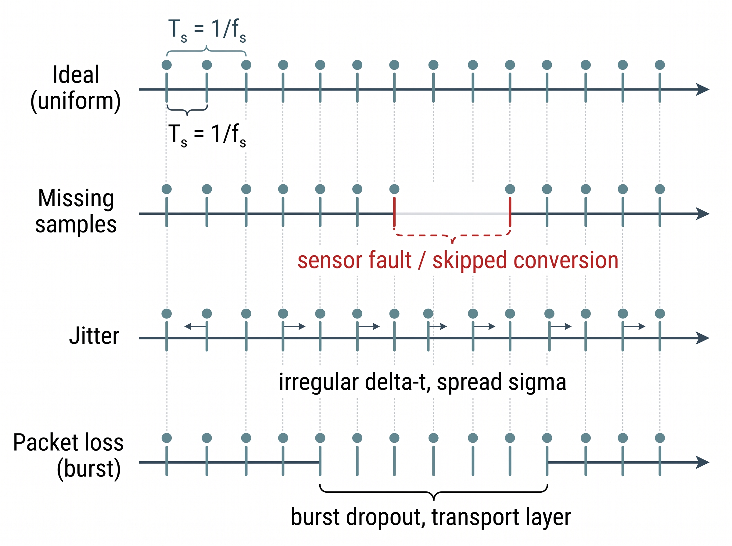
The three failure modes differ in cause even when they look alike in a plot. Missing samples means the underlying acquisition produced fewer readings than the nominal rate implies. An analog-to-digital converter (ADC) skipped a conversion, a sensor entered a fault state, or a firmware watchdog reset the chip mid-stream. The timeline has a hole. Jitter means the samples exist but their spacing is irregular: the intended interval is \(T_s = 1/f_s\), yet the actual interval \(\Delta t_n = t_n - t_{n-1}\) fluctuates. We summarize jitter by the standard deviation of those intervals, \(\sigma_{\Delta t}\), and by the peak-to-peak spread. Packet loss is a transport-layer phenomenon. The sensor measured correctly, but the bytes never reached your process: a corrupted radio frame, a dropped User Datagram Protocol (UDP) datagram, or a ring buffer that overwrote unread data. From the consumer's side packet loss looks like missing samples. Yet it arrives in characteristic bursts, and the protocol layer can often recover it, which pure sensor faults cannot. In short: a missing sample you have flagged is still data, while a missing sample you have hidden is a lie your model will believe. Figure 3.4.2 illustrates the taxonomy of temporal defects: missing samples vs jitter vs packet loss.

Why the pattern of missingness matters

Naming which of the three defects you face tells you what broke, but not how badly it will hurt; that severity is set by the pattern of the gaps, not merely by their presence. Borrowing the standard statistical taxonomy, missing data is missing completely at random (MCAR) when the dropout is independent of everything, missing at random (MAR) when it depends on observed covariates, and missing not at random (MNAR) when it depends on the unobserved value itself. This distinction is not academic. A pulse oximeter that drops readings precisely when the patient moves (motion also being what makes the reading dangerous) is MNAR: the gaps are correlated with the events you care most about. Imputing those gaps with the local mean will systematically erase the very episodes your model is meant to catch, and no amount of downstream accuracy on clean segments will reveal the bias. (This is why a 2 percent MNAR loss landing on the events you care about can wreck a detector that shrugs off a 20 percent MCAR loss spread across quiet stretches.) Characterizing whether your gaps are MCAR, MAR, or MNAR is a prerequisite for choosing any repair strategy, and it directly shapes the leakage-safe splits you will build in Chapter 5.

Measuring defects from timestamps

A classifier that quietly ingests a corrupted stream does not throw an error; it just ships wrong predictions in the field, and every repair choice and quality gate downstream inherits its trust from whether you quantified the damage first. You cannot repair what you have not measured. Given a vector of arrival timestamps, three numbers tell you almost everything: the distribution of inter-sample intervals \(\Delta t_n\), the count and duration of gaps (intervals exceeding a threshold such as \(1.5\,T_s\)), and the delivery ratio (received samples divided by expected samples over a window). The code below computes all three and, crucially, produces an explicit boolean missingness mask on a uniform reference grid rather than silently filling the holes. Figure 3.4.1 shows this alignment: jittered arrival timestamps are snapped to the nearest slot of a uniform grid, and the slots that no timestamp reaches become explicit holes in the boolean mask.

The delivery ratio is precisely the count of samples you actually received divided by the count the nominal rate says you should have received over the same interval, \(N_\text{obs} / N_\text{expected}\) where \(N_\text{expected} = \lfloor (t_{-1} - t_0)/T_s \rfloor + 1\); it is the single scalar that tells you how much of the promised timeline reached your process. It matters because it is a cheap, unit-free health gauge you can compute continuously and alarm on before any modeling begins. The mechanism is a simple ratio, so its one weakness is bluntness: a delivery ratio hides where the losses fell, which is why you pair it with the gap count and the boolean mask rather than trusting it alone. Reach for the delivery ratio when you need a fast per-window quality score for dashboards or gating; reach for the full mask when a downstream stage must know exactly which slots are empty.

import numpy as np

def profile_stream(timestamps, fs_nominal):
    """Diagnose jitter, gaps, and delivery ratio from arrival timestamps."""
    t = np.asarray(timestamps, dtype=float)
    dt = np.diff(t)
    Ts = 1.0 / fs_nominal

    jitter_std = dt.std()                      # timing irregularity, seconds
    gap_mask = dt > 1.5 * Ts                   # intervals that skipped samples
    n_missing = int(np.round((dt[gap_mask] / Ts - 1).sum()))
    expected = int(np.round((t[-1] - t[0]) / Ts)) + 1
    delivery_ratio = len(t) / expected

    # Build a uniform grid and a mask marking which grid slots were observed.
    grid = t[0] + np.arange(expected) * Ts
    idx = np.clip(np.round((t - t[0]) / Ts).astype(int), 0, expected - 1)
    observed = np.zeros(expected, dtype=bool)
    observed[idx] = True                       # True = real sample, False = hole

    return dict(jitter_std=jitter_std, n_missing=n_missing,
                delivery_ratio=delivery_ratio, grid=grid, observed=observed)

# Simulate a 50 Hz stream with jitter and a 1-second dropout burst.
rng = np.random.default_rng(0)
Ts = 1 / 50
clean = np.arange(0, 10, Ts)
jittered = clean + rng.normal(0, 0.002, clean.size)     # 2 ms RMS jitter
kept = jittered[(jittered < 4.0) | (jittered > 5.0)]     # drop 1 s of packets

p = profile_stream(kept, fs_nominal=50)
print(f"jitter RMS   : {p['jitter_std']*1e3:5.1f} ms")
print(f"missing count: {p['n_missing']}")
print(f"delivery     : {p['delivery_ratio']*100:5.1f} %")

Running it on the simulated stream reports roughly 2 ms of jitter, about 50 missing samples across the one-second dropout, and a delivery ratio near 90 percent. The mask is the deliverable that matters: it travels with the data and lets every later stage decide, explicitly, how to treat the holes.

Repair strategies, and when to trust them

Once holes are marked, you have four broad options, in ascending order of assumption. Leave them: many models, from the Kalman filter to modern attention, can consume a mask and skip absent inputs. A Kalman update, covered in Chapter 9, handles a missing measurement by running the prediction step alone and letting uncertainty grow. Interpolate: linear or spline fills are cheap and adequate for short gaps in slowly varying signals, but they fabricate high-frequency content and will fool a spectral feature extractor. Filter-based reconstruction: model-aware smoothing, the subject of Chapter 6, respects the signal's bandwidth when bridging gaps. Learned imputation: powerful, but it can hallucinate plausible values and, worse, leak information if fit on data that overlaps your evaluation set. The golden rule: interpolate for visualization freely, but never let an imputed value enter a training label or a safety-critical decision without a flag that says it was invented.

What's Next

Section 3.5 turns from the timing of samples to their values: how quantization and compression trade bits for fidelity, why an 8-bit ADC and a lossy codec each impose their own noise floor, and how to reason about the distortion budget before it silently caps what any downstream model can perceive.