Section 4.3: Bayesian inference and priors

"You gave me three noisy readings and asked what I believe. I already believed something before the first one arrived; the readings only told me how much to change my mind."
A Well-Calibrated AI Agent

Why this section matters

A sensor rarely gives you enough data to answer confidently on its own. A wearable sees three heartbeats before it must report a rate; a cold-start localizer has one range measurement; a fresh thermistor (a temperature-sensitive resistor used to measure temperature) off the line has a factory curve and nothing else. In every case you are not starting from zero: you already know that a resting heart rate is roughly 60 beats per minute, that a car cannot teleport between frames, that a thermistor's bias is small. Bayesian inference is the arithmetic of combining that prior knowledge with incoming evidence in the correct proportions. It is the single idea underneath Kalman filters, particle filters, sensor fusion, and modern uncertainty quantification, so it earns a careful treatment here before the rest of the book leans on it.

This section assumes you are comfortable with the random variables, densities, and expectations from Section 4.1 and with the likelihood and maximum-likelihood estimation (MLE) developed in Section 4.2. Where 4.2 asked "which parameter best explains the data," this section asks the fuller question: "given the data and what I already knew, what is my full belief about the parameter, uncertainty included." We keep the book's notation: a hidden quantity of interest is $\theta$ (a sensor bias, a state, a heart rate), the observed measurements are $x$, and the measurement model that links them was introduced as $x = h(\theta) + \eta$ in Chapter 2.

Bayes' theorem as a belief-update rule

Get the balance between prior knowledge and fresh evidence wrong and a wearable will either ignore a genuine spike in your heart rate or chase every sensor glitch as though it were real. Bayes' theorem is the one line of algebra that sets that balance, and it follows directly from the definition of conditional probability:

$$ p(\theta \mid x) \;=\; \frac{p(x \mid \theta)\, p(\theta)}{p(x)} \;\propto\; \underbrace{p(x \mid \theta)}_{\text{likelihood}}\;\underbrace{p(\theta)}_{\text{prior}}. $$

Read it right to left. The prior $p(\theta)$ is what you believe about $\theta$ before this measurement. The likelihood $p(x \mid \theta)$, the same object you maximized in 4.2, scores how well each candidate $\theta$ explains the data $x$. Their product, renormalized by the evidence $p(x)=\int p(x\mid\theta)p(\theta)\,d\theta$, is the posterior $p(\theta\mid x)$: your updated belief. The proportionality on the right is what you actually compute with, because the evidence is just the constant that makes the posterior integrate to one. Figure 4.3.1 traces this same multiply-then-normalize flow as a diagram: two inputs, one combination, one rescaling, one belief out.

The evidence term: not just bookkeeping

That normalizing denominator, the evidence $p(x)$, is itself a meaningful quantity rather than mere bookkeeping: it is the probability the model assigns to the observed data after averaging over every possible $\theta$, which is precisely why it is the currency for comparing whole models instead of parameter values. Mechanically it is obtained by integrating (or summing) the numerator $p(x\mid\theta)p(\theta)$ over all $\theta$, which is why closed-form posteriors are prized and why an intractable evidence integral forces the sampling methods later in this chapter. You can ignore it whenever you only need the shape of the posterior over $\theta$, as in ordinary parameter estimation, but you must compute it the moment you want to score one model against another, as in Bayesian model selection.

The posterior is a full distribution, not a point, so it carries both a best guess and a calibrated spread. That makes Bayesian inference the natural home for the aleatoric-versus-epistemic split of Section 4.4: the likelihood width encodes irreducible sensor noise, while the posterior width over $\theta$ encodes how far the data has pinned down the unknown. In short: a Bayesian belief is just what you knew multiplied by what you saw, renormalized so it still sums to one.

Figure 4.3.1. Bayes' theorem as a belief-update pipeline. The prior and the likelihood are multiplied, the product is rescaled by the evidence p(x) so it integrates to one, and the result is the posterior. The heavier border on the posterior marks it as the quantity the update produces.

The prior is not optional; it is only sometimes explicit

Maximum likelihood is Bayesian inference with a flat prior. Maximizing $p(x\mid\theta)$ is the same as maximizing $p(x\mid\theta)p(\theta)$ when $p(\theta)$ is constant. So MLE from Section 4.2 already assumed a prior; it just assumed the least defensible one, that every value of $\theta$ is equally plausible, including a resting heart rate of 5 or 500 beats per minute. Choosing a prior deliberately is not adding bias where there was none. It is replacing an accidental, usually indefensible prior with a stated, defensible one.

Priors: what to encode, why, and how much they cost

A prior encodes structure you know before seeing this particular data. Three kinds recur: physical bounds (a probability lies in $[0,1]$, a distance is non-negative), physics (a vehicle's acceleration is bounded, so its state cannot jump), and history (last year's calibration, the population distribution of resting heart rates). The practical question is always how strong to make it. You measure a prior's strength in pseudo-observations. A Gaussian prior with variance $\tau^2$ on a quantity measured at per-sample noise $\sigma^2$ is worth about $\sigma^2/\tau^2$ real measurements. Make it too weak and you throw away hard-won knowledge, forcing the sensor to relearn physics from every cold start. Make it too strong and the prior overrides the evidence the data was trying to deliver, so a genuinely fast heart rate gets dragged back toward 60.

Once you have settled how strong to make the prior, the next practical concern is how to fold it into the data cheaply, without evaluating an intractable integral. The mechanically convenient case is a conjugate prior: a prior whose functional form is preserved by the update, so the posterior is the same family with updated parameters and no integral to evaluate. In practice, two conjugate pairs cover most of what a sensing engineer typically needs. For a Gaussian measurement with known noise variance, a Gaussian prior on the mean yields a Gaussian posterior. For a binary event counted over trials (a fall detector firing, a beat classified as ectopic), a Beta prior on the success probability plus Binomial counts yields a Beta posterior. The Gaussian-Gaussian case is precisely the update rule that, run recursively over time, becomes the Kalman filter of Chapter 9.

The Gaussian-Gaussian posterior mean is worth memorizing, because it shows exactly how prior and data trade off. With prior $\theta\sim\mathcal{N}(\mu_0,\tau^2)$ and $n$ readings of mean $\bar{x}$ at noise $\sigma^2$:

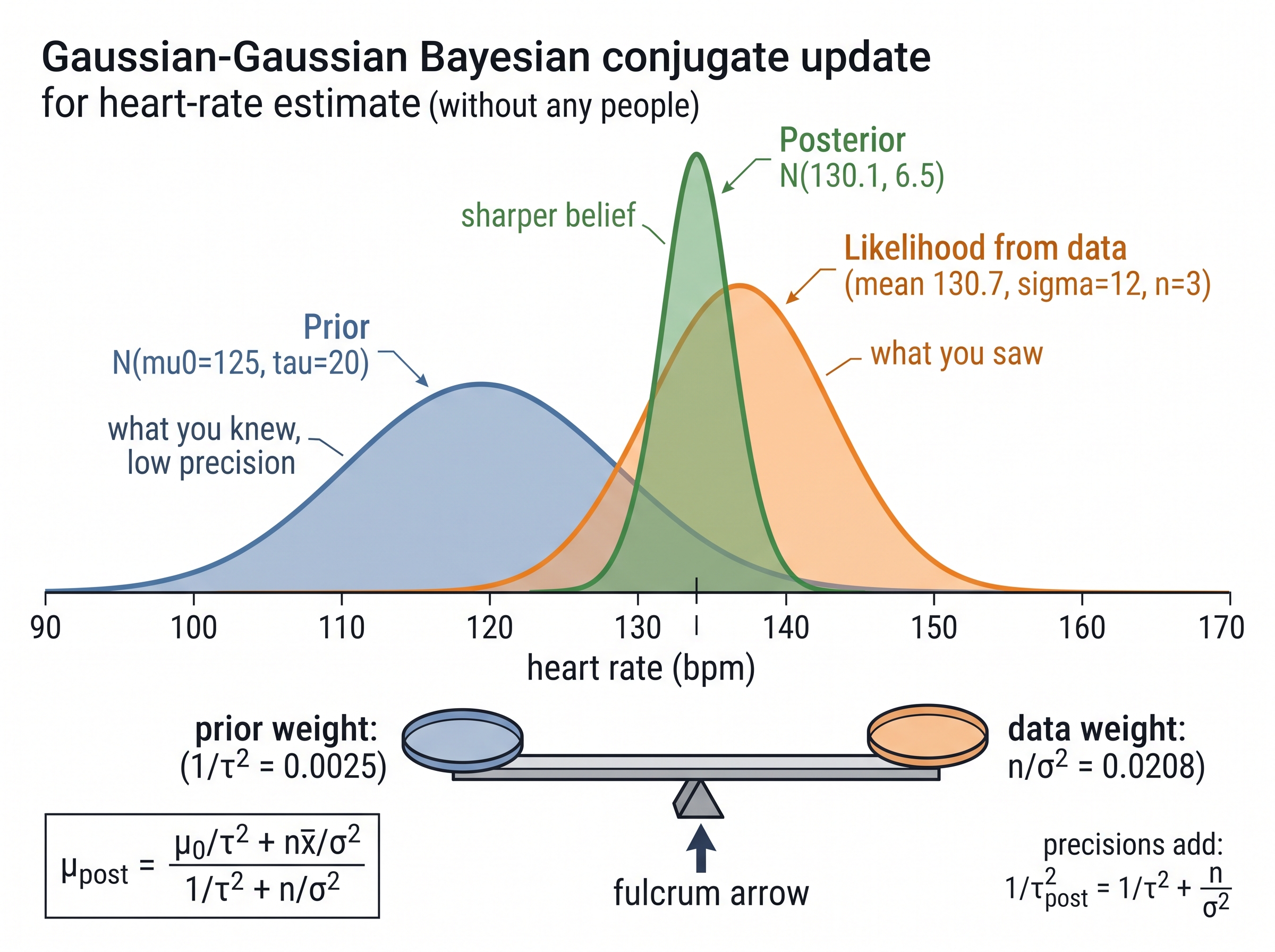
$$ \mu_{\text{post}} \;=\; \frac{\tfrac{1}{\tau^2}\,\mu_0 \;+\; \tfrac{n}{\sigma^2}\,\bar{x}}{\tfrac{1}{\tau^2} + \tfrac{n}{\sigma^2}}, \qquad \frac{1}{\tau_{\text{post}}^2} \;=\; \frac{1}{\tau^2} + \frac{n}{\sigma^2}. $$

The posterior mean is a precision-weighted average of the prior mean and the data mean, and precisions (inverse variances) add, since each independent reading contributes its own certainty. As $n$ grows, the data term dominates and the posterior converges to the MLE, which is why a well-chosen prior helps most exactly when data is scarce and fades gracefully when data is plentiful. Figure 4.3.2 illustrates the Gaussian-Gaussian conjugate update as precision-weighted fusion of prior and data.

Gaussian-Gaussian conjugate update as precision-weighted fusion of prior and data — Figure 4.3.2: The Gaussian-Gaussian conjugate update as precision-weighted fusion: a broad low-precision prior and a sharper data likelihood combine into a narrower posterior whose mean is the precision-weighted average and whose precision is the sum of the two.

Checkpoint

So far: a prior's strength is measured in pseudo-observations, a conjugate prior keeps the posterior in the same family so no integral is needed, and the Gaussian-Gaussian posterior mean is just a precision-weighted average of the prior and the data.

Step-Through: Beta-Binomial conjugate update

Trace the other workhorse conjugate pair with a tiny fall-detector example, one update at a time, using actual numbers. We track the belief about a fall detector's per-event false-alarm probability $p$, starting from a weak prior Beta$(\alpha,\beta)=\text{Beta}(2,8)$ (prior mean $2/10=0.20$), and feed it a stream of outcomes where 1 means a false alarm fired.

Start. $\alpha=2,\ \beta=8$. Prior mean $=\alpha/(\alpha+\beta)=2/10=0.200$.
Observe a false alarm (1). A success increments $\alpha$: $\alpha=3,\ \beta=8$. Mean $=3/11=0.273$. The single alarm pushed the belief up.
Observe a clean event (0). A failure increments $\beta$: $\alpha=3,\ \beta=9$. Mean $=3/12=0.250$.
Observe clean, clean (0, 0). $\beta$ grows twice: $\alpha=3,\ \beta=11$. Mean $=3/14=0.214$, sliding back toward the prior as evidence of reliability accumulates.
Read off the spread. The final Beta$(3,11)$ has standard deviation $\sqrt{\alpha\beta/[(\alpha+\beta)^2(\alpha+\beta+1)]}=\sqrt{33/(196\cdot15)}\approx0.106$, a calibrated uncertainty band the raw count $1/4=0.25$ could never report.

Notice the whole update was bookkeeping on two integers: successes add to $\alpha$, failures add to $\beta$, and no integral was ever evaluated. That is exactly the payoff of conjugacy.

Mental Model

Picture two friends proposing a meeting time. One is fairly sure it should be around 1 pm but often misremembers; the other insists on 2 pm and is almost never wrong. You do not naively split the difference at 1:30, you land much closer to 2 pm, because you weight each opinion by how trustworthy it is. "Precision" is exactly that trustworthiness (the inverse of how far off each source tends to be), the posterior mean is the confidence-weighted compromise between the two, and the fact that precisions add captures the everyday intuition that two independent trustworthy opinions leave you more certain than either one alone.

Common Misconception

The misconception is that "because the data eventually overwhelms the prior, the choice of prior never really matters." That reassurance only holds in the large-$n$ limit; in the scarce-data regime where you actually reach for Bayes (a cold start, a single noisy reading) the prior materially sets the answer, and a badly chosen prior yields a badly wrong posterior that the three samples you happen to have will not rescue.

Cold-starting a wearable heart-rate estimate

A wrist optical heart-rate monitor comes out of a tunnel with the photoplethysmography (PPG) signal briefly corrupted; it recovers three clean inter-beat intervals implying rates of 132, 119, and 141 beats per minute, so $\bar{x}=130.7$, each with per-reading noise $\sigma=12$. A pure-MLE device reports 130.7 and, if one interval were an artifact, could swing wildly. Now add a mild prior from the user's own history: their exercise heart rate this week has centered at $\mu_0=125$ with $\tau=20$. Precisions give the data weight $3/12^2=0.0208$ and the prior weight $1/20^2=0.0025$, so $\mu_{\text{post}} = (0.0025\cdot125 + 0.0208\cdot130.7)/0.0233 \approx 130.1$ with a posterior standard deviation of about 6.5. The prior barely moved the estimate because three clean beats already outweigh it eight to one, which is the correct behavior: the prior stabilizes the first uncertain sample and then politely steps aside. Push the same math into the recovery instant with only one noisy reading and the prior does real work, keeping the reported rate physiological instead of tracking a single glitch.

The following snippet implements the conjugate update directly, so you can watch the posterior tighten as readings arrive.

import numpy as np

def gaussian_update(mu0, tau2, readings, sigma2):
    """Sequential Gaussian-Gaussian posterior for a scalar mean."""
    mu, prec = mu0, 1.0 / tau2          # track mean and precision (1/variance)
    for x in readings:
        prec_new = prec + 1.0 / sigma2  # precisions add
        mu = (prec * mu + (1.0 / sigma2) * x) / prec_new
        prec = prec_new
    return mu, 1.0 / prec               # posterior mean, posterior variance

mu, var = gaussian_update(125.0, 20.0**2, [132, 119, 141], 12.0**2)
print(f"posterior mean {mu:.1f} bpm, std {np.sqrt(var):.1f} bpm")
# posterior mean 130.1 bpm, std 6.5 bpm

A twelve-line sequential Gaussian-Gaussian update: each reading adds its precision and pulls the mean toward the data, reproducing the wearable heart-rate numbers from the practical example above.

When conjugacy runs out, let a sampler carry the posterior

Conjugate updates are exact but only exist for a handful of prior-likelihood pairs. The moment your measurement model is nonlinear (a distance that depends on the square root of a state) or your prior is non-Gaussian, the evidence integral $p(x)$ has no closed form and the hand-rolled update above no longer applies. A probabilistic programming library replaces roughly 40 to 60 lines of bespoke sampler code with a model declaration:

import pymc as pm

with pm.Model() as m:
    theta = pm.Normal("theta", mu=125.0, sigma=20.0)     # the prior
    pm.Normal("obs", mu=theta, sigma=12.0,               # the likelihood
              observed=[132, 119, 141])
    idata = pm.sample(1000, progressbar=False)           # posterior samples

Declaring the same heart-rate model in PyMC; the library handles the sampler, tuning, convergence diagnostics, and posterior summarization that a from-scratch Markov chain Monte Carlo (MCMC) routine would spell out by hand.

The library handles the sampling algorithm, step-size tuning, convergence checks, and posterior summaries internally. You get the same posterior mean and standard deviation as the conjugate formula here, but the identical code now scales to nonlinear measurement models where no closed form exists, the regime that Monte Carlo methods in Section 4.7 and particle filtering in Chapter 10 are built to handle.

Real-World Application: spacecraft navigation

NASA's Deep Space Network navigation for missions like Mars 2020 fuses sparse, noisy Doppler and range measurements into a spacecraft trajectory using exactly the prior-times-likelihood update of this section, run recursively as a Kalman filter. The prior is the orbit-propagation model (gravity and thrust tell you where the craft should be before the next radio contact), and each Doppler reading is a likelihood that tightens the posterior on position and velocity, which is what lets a lander hit a target ellipse tens of millions of kilometers away from a handful of measurements.

The theorem that found a lost submarine

In 1968 the submarine USS Scorpion vanished in the Atlantic with no distress signal and only a vague last position. Rather than search a hopeless expanse, John Craven's team built a Bayesian prior by polling submarine experts on competing scenarios, laid it as a probability map over the seabed, and updated it as each fruitless search pass ruled out squares. The wreck was reportedly found within a few hundred meters of the posterior's peak, and the same "search theory" had two years earlier recovered a lost hydrogen bomb off the coast of Spain (Palomares, 1966), a striking case of a two-and-a-half-century-old formula outperforming intuition when data was almost nonexistent.

Research Frontier

When even a general sampler is too slow (a sensor that must emit a fresh posterior at every timestep), the frontier is amortized simulation-based inference: train a neural network once on simulated $(\theta, x)$ pairs so that inference at run time is a single forward pass, with no likelihood evaluation and no per-query Markov chain. Gloeckler et al.'s "All-in-one simulation-based inference" (ICML 2024) introduces the Simformer, a transformer-based architecture that amortizes the posterior over arbitrary conditionals of a probabilistic model, so one trained network can answer many different Bayesian queries about a sensor system without re-running inference for each.

Reporting a belief: MAP, posterior mean, and credible intervals

A posterior is a distribution, but a device often has to emit one number. Three summaries dominate. The maximum a posteriori (MAP) estimate is the posterior mode, $\arg\max_\theta p(\theta\mid x)$; it is MLE with the prior's regularizing pull, and for a Gaussian posterior it coincides with the mean. The posterior mean minimizes expected squared error and is the standard choice when the cost of being wrong grows with the square of the error. A credible interval, for example the central region containing 95 percent of posterior mass, is the honest uncertainty report, and unlike a frequentist confidence interval (one whose 95 percent refers to the long-run success rate of the procedure, not a probability about this particular parameter) it means exactly what a newcomer expects: given the data and prior, there is a 95 percent probability the parameter lies inside it.

MAP also exposes the bridge to everyday deep learning. Maximizing $\log p(x\mid\theta) + \log p(\theta)$ is a data-fit term plus a penalty term, and a zero-mean Gaussian prior makes that penalty a sum of squares. That is L2 weight regularization, and a Laplace (double-exponential) prior is L1. Every time a model is trained with weight decay, a prior is being asserted, whether or not anyone says so. This is the same identity the calibration and uncertainty methods of Chapter 18 build on.

Exercise

A vibration monitor on a pump classifies each of $n=8$ startup cycles as "faulty" or "normal" and observes 2 faults. Model the fault probability $p$ with a Beta$(\alpha,\beta)$ prior. (a) Using the reliability team's belief that faults are rare, encoded as Beta$(2, 20)$, compute the posterior after the 8 cycles (recall the Beta-Binomial posterior is Beta$(\alpha + \text{faults}, \beta + \text{non-faults})$). (b) Report the posterior mean $\alpha'/(\alpha'+\beta')$ and compare it with the raw MLE of $2/8$. (c) How many additional clean cycles would it take for the posterior mean to fall below 0.10, and what does that tell you about the prior's strength in pseudo-observations?

Self-check

Why is maximum-likelihood estimation a special case of Bayesian inference, and which prior does it silently assume?
In the Gaussian-Gaussian posterior mean, what quantity determines how much weight the data receives relative to the prior, and what happens to that weight as the number of readings grows?
A colleague reports a 95 percent credible interval and a 95 percent confidence interval as if they mean the same thing. State the difference in one sentence.

When to reach for Bayes, and when not to

Reach for Bayes in three cases: when data is scarce relative to the number of unknowns, when you genuinely hold prior knowledge worth encoding (physics, calibration history, population statistics), and above all when you must report calibrated uncertainty rather than a bare point estimate. A device that acts on its own confidence needs that confidence to be honest. The cost is real: you must choose a prior and, outside conjugate cases, pay for approximate inference. When data is abundant and a point estimate suffices, MLE from Section 4.2 is cheaper and the prior washes out anyway. The recursive form of the Gaussian update seen here drives the entire state-estimation part of this book. Its multi-sensor generalization, where each sensor contributes a likelihood and priors propagate between them, is the subject of Chapter 49 on probabilistic fusion.

Try It: Watch a prior fade as data arrives

Reproduce, then stress-test, the prior-versus-data tradeoff on your own laptop with NumPy and Matplotlib in about twenty minutes.

Copy the twelve-line gaussian_update function above and set a deliberately wrong prior, $\mu_0=125$ with $\tau=20$, while drawing "true" readings from np.random.normal(150, 12, size=50).
Loop n from 1 to 50, calling the update on the first n readings, and record the posterior mean and standard deviation at each step.
Plot posterior mean versus n with a shaded $\pm 1$ standard-deviation band, and overlay horizontal lines at the prior mean 125 and the true mean 150.
Rerun with a much stronger prior ($\tau=3$) and a much weaker one ($\tau=100$), and watch how many readings each version needs before its posterior mean crosses 145.
Report the smallest n at which the posterior mean exceeds 145 for each $\tau$; that count is the prior's strength in pseudo-observations made visible.

Lab: Conjugate posterior versus a real sampler

Goal. Convince yourself, empirically, that the closed-form Gaussian-Gaussian update and a general-purpose MCMC sampler agree on the same posterior, then watch where conjugacy breaks and only the sampler survives. Budget 20 to 30 minutes.

Tools. Python with numpy, matplotlib, and pymc (pip install pymc); the ten-line gaussian_update function from this section.

Baseline. Simulate 10 readings from np.random.normal(150, 12, size=10). Compute the conjugate posterior mean and standard deviation with gaussian_update(125, 20**2, readings, 12**2).
Sampler. Declare the identical model in PyMC (Normal("theta", 125, 20) prior, Normal("obs", theta, 12, observed=readings)) and call pm.sample(). Compare the sampled posterior mean and standard deviation to the closed form; they should match within Monte Carlo error.
What to vary. Sweep the prior width $\tau \in \{3, 20, 100\}$ and the sample size $n \in \{1, 3, 10, 50\}$. Overlay the conjugate posterior density and a histogram of the PyMC samples for each combination.
Break conjugacy. Replace the likelihood mean with a nonlinear link, mu = pm.math.sqrt(theta), so the observation model is no longer Gaussian in $\theta$. The conjugate formula no longer applies; rerun the sampler and inspect the now-skewed posterior.
What to observe. Confirm that (a) closed form and sampler agree exactly in the linear-Gaussian case, (b) the posterior narrows predictably as $n$ grows and as $\tau$ shrinks, and (c) the nonlinear case yields an asymmetric posterior that no add-the-precisions shortcut could have produced, which is the concrete reason the sampling methods of Section 4.7 exist.

What's Next

In Section 4.4, we split the uncertainty this section quantified into its two irreducible kinds: aleatoric uncertainty, the noise the world will never let you remove, and epistemic uncertainty, the ignorance that more data can. The posterior width you just learned to compute is where that distinction becomes operational, and it is the thread that runs through every calibration, fusion, and safety chapter that follows.