Aleatoric vs epistemic uncertainty (introduced early, used everywhere)

"I am 90 percent sure. The remaining 10 percent is split between the world being noisy and me being ignorant, and those two demand opposite fixes."

A Self-Aware AI Agent

The prerequisites are random variables, expectation, and variance from Section 4.1, the estimator language of Section 4.2, and the posterior-over-parameters view of Section 4.3. If you want the physical origin of measurement noise (why the aleatoric floor exists at all), Chapter 2 derives it from sensor physics.

Two sources of doubt, one predictive distribution

Formally, both flavors live inside a single predictive distribution but enter through different doors. Suppose a model with parameters \(\theta\) predicts an output \(y\) from an input \(x\). The parameters themselves are uncertain, described by a posterior \(p(\theta \mid \mathcal{D})\) learned from data \(\mathcal{D}\). The full predictive distribution marginalizes over that posterior (averages the prediction across every plausible \(\theta\), weighting each by how much the data supports it):

The inner term \(p(y \mid x, \theta)\) is the aleatoric part: even if you knew \(\theta\) exactly, \(y\) would still scatter because the world and the sensor are noisy. The spread of \(p(\theta \mid \mathcal{D})\) is the epistemic part: the width of your belief about the model itself. The law of total variance makes the split exact for a scalar output:

Read it aloud: total variance equals the average noise across plausible models, plus the disagreement between those models. The first term does not shrink as \(\mathcal{D}\) grows; the second collapses toward zero as the posterior concentrates. That single asymmetry is the whole reason we bother to separate them. In short: one kind of doubt dissolves with more data and the other never will, so before you spend a dollar, first ask which one you are looking at.

Why the distinction changes what you do next

The two flavors route to different interventions, and getting the routing wrong wastes budget. High aleatoric uncertainty says the signal-to-noise ratio is the bottleneck: add sensor redundancy, average longer windows, cool the detector, improve the analog front end, or fuse a complementary modality. No amount of retraining helps, because the label genuinely is ambiguous given the input. High epistemic uncertainty says the model is out of its depth: gather data from the missing regime, widen the training distribution, or fall back to a safe default until you do. This signal drives two techniques. Active learning labels the points the model is most epistemically unsure about. Out-of-distribution (OOD) detection watches for the epistemic spike on inputs unlike anything in \(\mathcal{D}\).

Having routed the epistemic case to its interventions, return to the aleatoric side, which is not a single quantity either. Aleatoric uncertainty further splits into homoscedastic (constant across inputs, like a fixed quantization step) and heteroscedastic (input-dependent, like a heart-rate estimate that degrades during vigorous motion). Heteroscedastic modeling matters for real sensors because noise is rarely uniform: a lidar return is crisp at 5 m and mushy at 80 m, and a good model should say so per point.

Estimating the split in practice

Get this approximation wrong and the cost is concrete: a self-driving perception stack that cannot separate a genuinely occluded pedestrian (aleatoric, brake now) from an unfamiliar object (epistemic, hand back control) will either stop for phantoms or sail straight past real danger. So the estimator you pick here is not bookkeeping; it decides which of those two actions the vehicle takes. You rarely have the exact integral, so you approximate it. The dominant recipe is an ensemble (or its cheap cousin, Monte Carlo dropout): train several models, or sample several parameter settings, and look at how their predictions behave. Each member predicts both a mean \(\mu_m(x)\) and its own noise \(\sigma_m^2(x)\) (the heteroscedastic aleatoric head, the output branch of the network that predicts a separate noise level for each input). Then the two components fall straight out of the total-variance formula: the aleatoric estimate is the mean of the per-member variances, and the epistemic estimate is the variance of the per-member means.

Concretely, a deep ensemble is just several copies of the same network trained independently from different random initializations (and usually different data shuffles), so their predictions on a fresh input behave as samples from the posterior \(p(\theta \mid \mathcal{D})\) that you cannot integrate in closed form. It matters because that spread is the main practical window (alongside an explicit Bayesian posterior) onto epistemic uncertainty for modern networks: where the members agree the posterior is effectively tight, and where they diverge it is broad. Mechanically you train \(M\) models once, cache their weights, then at inference run all \(M\) forward passes and hand the outputs to the decomposition below; reach for a full ensemble when you can afford the \(M\)-fold compute and want the strongest estimates, and fall back to Monte Carlo dropout (one network, many stochastic forward passes) when you cannot pay for \(M\) separate trainings. Figure 4.4.1 traces how the \(M\) member outputs split into the two uncertainty components.

import numpy as np

# preds: shape (M, N) predicted means from M ensemble members over N inputs
# sigmas: shape (M, N) each member's predicted aleatoric std (heteroscedastic head)
def decompose_uncertainty(preds, sigmas):
    aleatoric = np.mean(sigmas ** 2, axis=0)      # avg noise across models
    epistemic = np.var(preds, axis=0)             # disagreement between models
    total = aleatoric + epistemic
    return aleatoric, epistemic, total

# toy: 5 members, one in-distribution point and one far-out point
preds  = np.array([[10.0, 3.0], [10.1, 7.0], [9.9, 1.0], [10.0, 9.0], [10.2, 4.0]])
sigmas = np.array([[0.5, 0.5], [0.5, 0.5], [0.5, 0.5], [0.5, 0.5], [0.5, 0.5]])
a, e, t = decompose_uncertainty(preds, sigmas)
print("aleatoric:", a.round(3))   # ~[0.25, 0.25] : same sensor-noise floor
print("epistemic:", e.round(3))   # ~[0.01, 7.8 ] : members agree, then wildly disagree

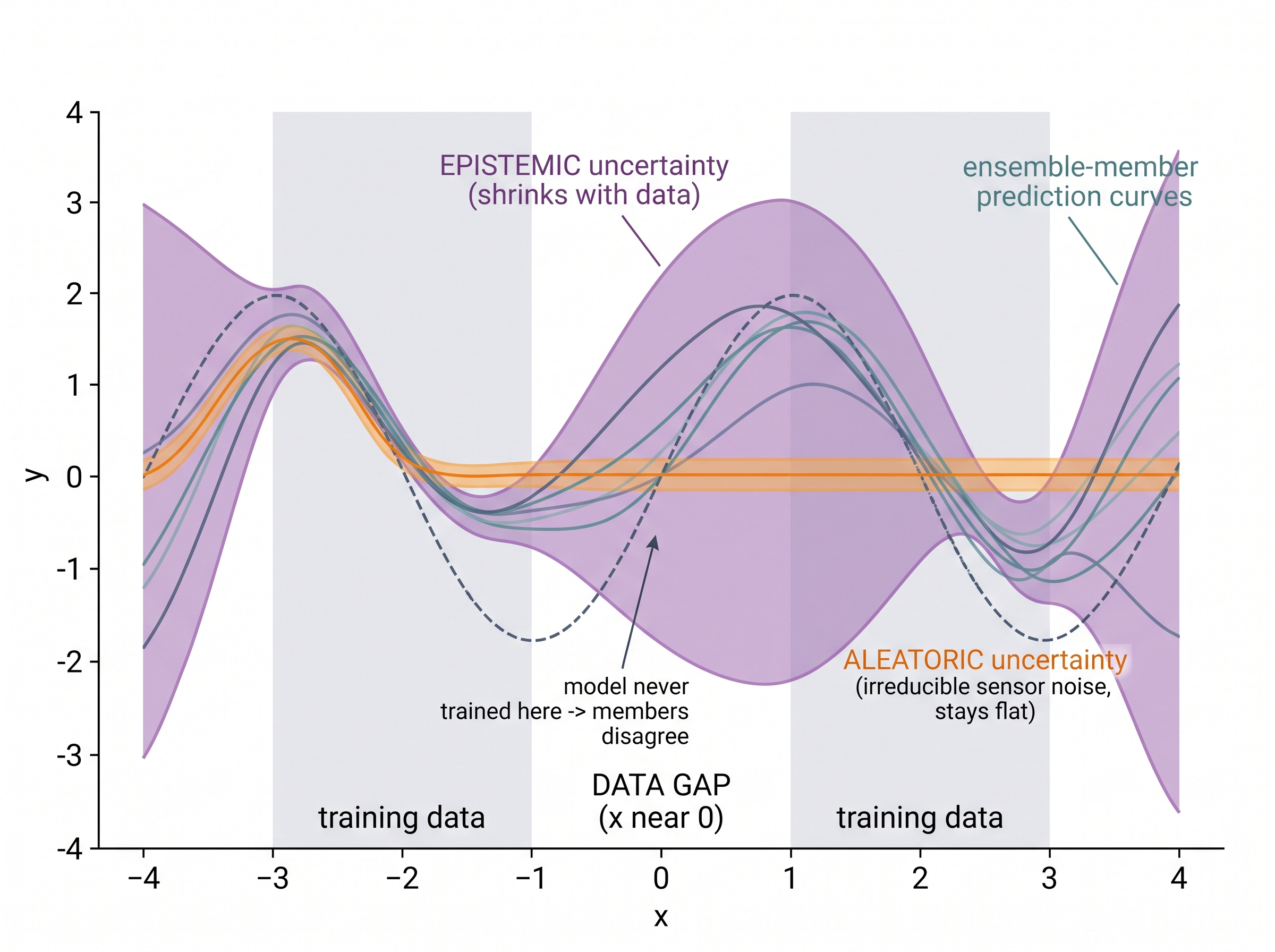
That snippet is the whole mechanism: aleatoric is the average of the noise, epistemic is the spread of the means. Agreement drives epistemic to near zero and leaves the irreducible sensor floor; scatter means the model has never seen this input. Chapter 66 turns that epistemic spike into a monitoring alarm. Figure 4.4.2 illustrates how epistemic uncertainty balloons in a data gap while aleatoric stays flat.

Where this split reappears in the rest of the book

This foundations chapter introduces aleatoric versus epistemic because the split is load-bearing everywhere downstream. Bayesian filters in Chapter 9 encode aleatoric sensor noise in the measurement covariance \(R\) and epistemic-like process uncertainty in \(Q\); mixing them up detunes the whole filter. Sensor fusion in Part X weights each modality by its aleatoric noise and drops a modality when its epistemic uncertainty says it is unreliable. Calibration and conformal prediction in Chapter 18 make these numbers honest. A stated 90 percent interval then contains the truth 90 percent of the time. Functional-safety arguments demand the split explicitly: a self-driving stack must distinguish "the fog is genuinely occluding this pedestrian" (aleatoric, slow down) from "this object looks like nothing in training" (epistemic, hand back control). Carry the vocabulary forward; you will use it in nearly every chapter that estimates anything.

What's Next

In Section 4.5, we quantify uncertainty itself with the tools of information theory: entropy measures how much doubt a distribution holds, and mutual information measures how much a new sensor reading is expected to remove. That is exactly the machinery that turns the epistemic uncertainty you just learned to isolate into a concrete, optimizable rule for deciding which measurement to take next.