Normalization and per-device calibration

"Two sensors reading the same world will still disagree. Normalization is how you argue them into a common language without whispering the test answers on the way."

A Diplomatic AI Agent

This section assumes you understand sensor bias, gain, and drift as physical quantities, developed in Chapter 2, and the leakage-safe split boundaries (device, user, site) from Section 5.4. Here we take windowed, split data and ask how to scale and calibrate it so that a model trained on one set of devices behaves on another. We deliberately treat model-output calibration (making predicted probabilities match observed frequencies) as a separate topic, covered in Chapter 18; the word "calibration" here means the hardware sense.

Why raw units mislead a model

What. Most sensor channels arrive in physical or raw-count units that mix three things: the signal, a per-device offset, and a per-device scale. We model a single reading as \(x = g\,(s + b) + \varepsilon\), where \(s\) is the true stimulus, \(b\) is a bias, \(g\) is a gain, and \(\varepsilon\) is noise. Why it matters. Gradient-based models typically converge poorly when channels span wildly different magnitudes. Feed an accelerometer in \(\pm 20\ \text{m/s}^2\) and a barometer in \(\sim 10^5\ \text{Pa}\) into the same network, and the barometer dominates every dot product until the optimizer laboriously rescales its own weights. (A barometer near \(10^5\) sitting next to an accelerometer near \(20\) is roughly a 5,000x magnitude gap, so the loss is effectively barometer-only until normalization levels the channels.) Worse, if \(b\) and \(g\) differ per device, a model that learned "class A sits near value 3.1" on the training devices will be wrong on a test device whose baseline sits at 3.4. How. Normalization fixes the magnitude problem; calibration fixes the per-device offset-and-gain problem. They are related but not the same operation, and conflating them is where subtle bugs live.

Normalization schemes and where the statistics come from

Pick the wrong scaler and a single vibration spike can quietly rescale an entire channel, teaching your model to key off a one-off artifact instead of the phenomenon; the choice below is not cosmetic, it decides what your network is even able to see. What. The workhorses are per-channel z-score (subtract mean, divide by standard deviation), min-max (rescale to \([0,1]\)), and robust scaling (subtract median, divide by interquartile range). For a channel \(c\), z-scoring is

where \(\mu_c\) and \(\sigma_c\) are estimated statistics. Robust scaling swaps in order statistics for the same job, \(\tilde{x}_c = (x_c - \text{med}_c)/\text{IQR}_c\), where \(\text{med}_c\) is the channel median and \(\text{IQR}_c\) is its interquartile range, so neither term moves when a lone spike lands in the tail. When to prefer which. Use z-score as the default for roughly symmetric signals; use robust scaling when outliers and spikes are common (vibration, electromyography (EMG) bursts), because a single clipping event can wreck a standard deviation; use min-max only when a signal has hard physical bounds and you truly want to preserve them. How, and the part everyone gets wrong. The statistics \(\mu_c, \sigma_c\) are learned parameters of your pipeline, so they must be estimated on the training split alone and then applied unchanged to validation and test. Estimating them over the full dataset lets the test set's mean and variance leak backward into training, which is exactly the failure Section 5.3 warns against.

Min-max, precisely. Min-max normalization linearly maps a channel onto a fixed interval with \(\tilde{x} = (x - x_{\min})/(x_{\max} - x_{\min})\), so the smallest observed value becomes 0 and the largest becomes 1 while every gap between them stays proportional. It matters because a bounded \([0,1]\) range keeps signals with real physical limits (a normalized pixel intensity, a percent-of-scale humidity reading) inside the span a bounded activation expects, and it does this through one assumption-free subtract-and-divide rather than any distributional estimate. Reach for it only when those limits are genuine and stable; prefer z-score or robust scaling when the extremes are noisy, because a single spike moves \(x_{\max}\) and silently rescales every other sample. In short: a normalizer is a model you fit, so let it look only where your model is allowed to look.

Per-device calibration: making devices speak the same units

Rescaling tames magnitude, but it never touches the physical reason two devices disagree about the very same input, and that is exactly where calibration takes over. What. Calibration removes the sensor-specific transfer function (the fixed input-to-output mapping a given unit imposes on top of the true signal) so that a known input maps to a known output on every unit. The classic two-point linear calibration solves for gain and offset from two reference stimuli \(s_1, s_2\) with measured responses \(x_1, x_2\): \(g = (x_2 - x_1)/(s_2 - s_1)\) and \(b = x_1 - g\,s_1\), then recovers \(\hat{s} = (x - b)/g\). Why it is separate from normalization. Normalization uses statistics of your data; calibration uses references from the physical world (a level surface for an inertial measurement unit (IMU), ice and boiling water for a thermistor, a zero-gas purge for a chemical sensor). You can calibrate each device with no labels at all, which is powerful, because it attacks device shift at its source rather than hoping the model averages it out. When you lack references. If you cannot bench-calibrate, per-device normalization is the pragmatic stand-in (a lighter-weight cousin of the instance normalization defined later in this section): compute each device's own baseline statistics (from a resting period, or a rolling window) and normalize each device by its own numbers. This needs no true \(g, b\), only that each device becomes internally consistent.

Instance normalization and the shift it defends against

That runtime bias tracker, which leans on a device's own recent statistics, points to a lighter-weight move you can make even when no resting baseline is available. What. You can normalize each window by its own statistics at inference time: subtract the window mean, divide by its per-channel standard deviation. This is instance normalization; its reversible form (normalize the input, then add the statistics back to the output) is the forecasting literature's reversible instance normalization. Why. It removes the slow per-window offset and scale shifts a global scaler cannot track, the very drift that breaks cross-device and cross-day generalization. When. Prefer it when shape carries the class and absolute level does not (activity recognition, many fault-detection tasks); avoid it when the level is the signal (a barometer for altitude, a thermometer for fever), where you would normalize away what you want to predict. Chapter 13 revisits this design space for deep models.

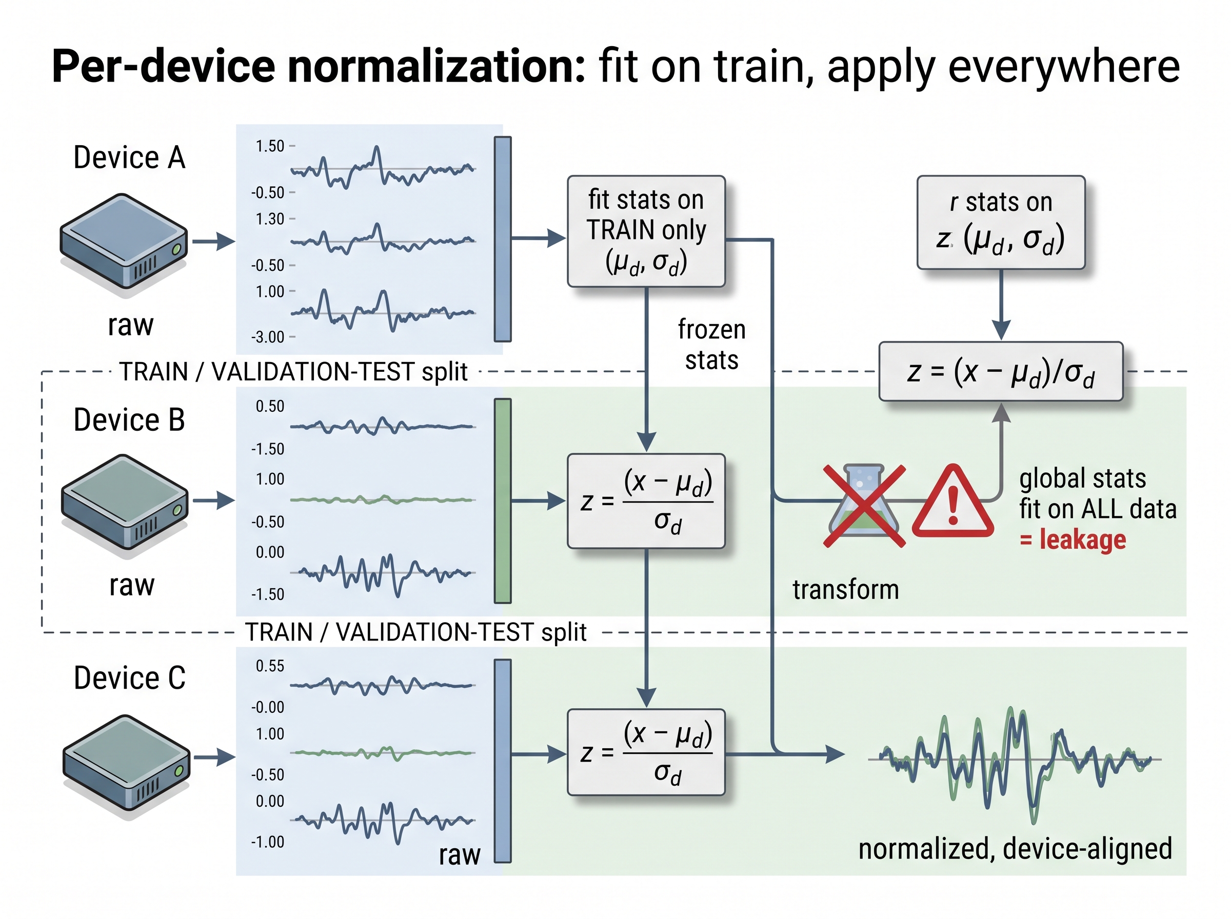
The leakage-safe fit and transform boundary diagrammed in Figure 5.5.1 makes the rule visual: statistics flow out of the training devices only, and no arrow ever runs backward from the held-out devices into the fitted scaler. The code below shows the same pattern end to end: fit a per-channel scaler on the training devices only, then apply a per-device baseline correction that each device computes from its own resting statistics. Note that nothing about the validation devices touches the fitted scaler's parameters.

import numpy as np

class LeakageSafeScaler:
    """Per-channel z-score fit on TRAIN groups only, plus per-device debias."""
    def fit(self, X_train):                    # X_train: (N, L, C) train windows
        flat = X_train.reshape(-1, X_train.shape[-1])
        self.mu = flat.mean(0)                  # (C,) learned on train ONLY
        self.sigma = flat.std(0) + 1e-8
        return self

    def transform(self, X, device_baseline=None):
        Xc = X.astype(np.float64)
        if device_baseline is not None:         # per-device offset removal
            Xc = Xc - device_baseline           # (C,) this device's own zero
        return (Xc - self.mu) / self.sigma

# Fit on training devices, freeze, then transform each device by ITS baseline.
scaler = LeakageSafeScaler().fit(X_train)       # never sees val/test devices
base_val = X_val_rest.mean((0, 1))              # this device's resting mean (C,)
X_val_norm = scaler.transform(X_val, device_baseline=base_val)
print(X_train.shape[-1], "channels; scaler frozen on train")

Normalization and calibration are the last preprocessing step before modeling and the one most likely to quietly corrupt an otherwise careful pipeline. Treat the scaler as a fitted model with a strict train-only fitting rule, keep hardware calibration distinct from data-statistics normalization, and push per-device corrections down to the device when its bias is private and time-varying. These habits are what let a model cross the gap from the devices it trained on to the ones it will actually run on.

What's Next

In Section 5.6, we turn from the signal side to the label side: annotation quality, weak and noisy labels, and the label delay that shifts your ground truth in time. A perfectly normalized dataset with sloppy labels still trains a sloppy model, and label noise is best treated as its own source of error.