"The test set exists to answer one question: what happens when something new walks in the door. If the door already knows the visitor, you asked a different question and reported the wrong answer."
A Disciplined AI Agent
The Big Picture
The previous section named the disease: leakage lets test information contaminate training and inflates your numbers. This section prescribes the cure that fixes most sensor leakage in one move: group-aware splitting. Instead of shuffling windows at random, you decide which real-world entity your model must generalize across, hold all of that entity's data on one side of the split, and never let it straddle. The entity might be a device, a wearer, a factory site, a recording session, or a physical machine. Choosing it correctly is typically among the highest-leverage decisions in your evaluation protocol, because it defines what "new" means for your deployed system. Choose it wrong and a model that has secretly memorized individuals will post a benchmark it can never reproduce in the field.
You cut the streams into windows back in Section 5.2 and learned every way they leak in Section 5.3; now picture shipping a model that scored 97% in the lab, watching it drop to a coin flip the instant a new patient is wheeled in, and discovering that the only thing standing between triumph and embarrassment was where you drew the line between train and test. This section turns that diagnosis into a construction procedure: we take a windowed, labeled dataset carrying entity identifiers and produce train, validation, and test partitions whose accuracy estimate matches the deployment question you actually care about.
The grouping unit is a modeling decision, not a default
A model that has quietly learned to recognize the wearer instead of the motion can post a near-perfect lab score and then collapse the moment a stranger straps on the sensor, and the whole difference traces to a single decision about how you group the data. What. A grouping unit is the entity across whose boundary your model must generalize at deployment. Every window belongs to exactly one value of that unit: this wearer, that machine, this recording session. A group-disjoint split then guarantees that all windows sharing a group value land entirely in train or entirely in test, never straddling the two. Why. Sensor data is riddled with nuisance signals that are constant within an entity and irrelevant to the label: a specific accelerometer's bias, one person's gait idiosyncrasy, a particular lathe's bearing hum, a room's acoustic reverberation. A random split scatters an entity's windows across train and test, so the model can lower its loss by recognizing the entity rather than the phenomenon. That shortcut evaporates the instant a genuinely new entity appears. In short: pick the entity your model must generalize across, keep every one of its windows on a single side of the split, and your accuracy finally means what it claims. Figure 5.4.2 illustrates random window split versus group-disjoint split (how leakage arises).
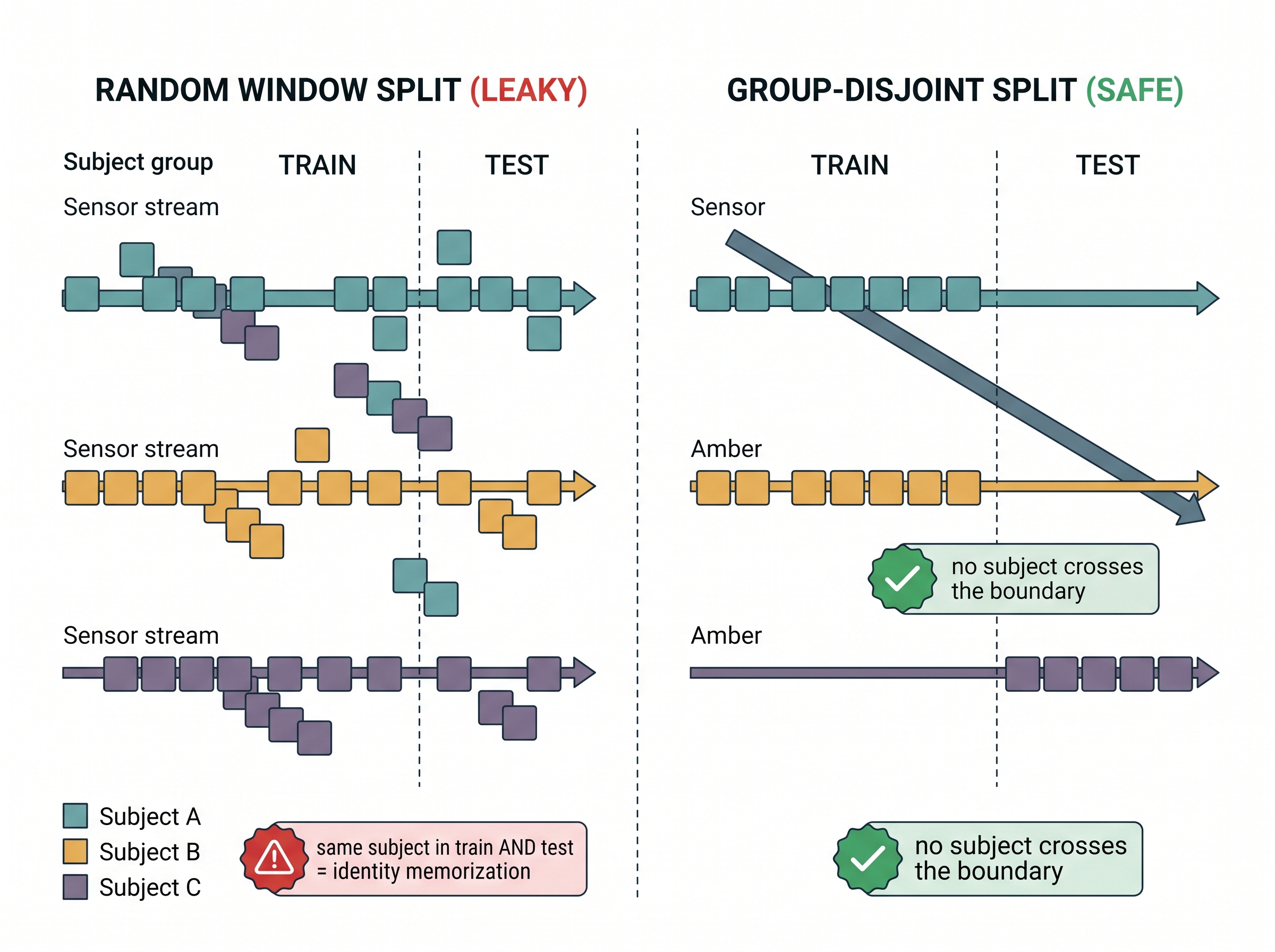
Mental Model
Picture a teacher grading anonymous essays who has quietly learned each pupil's handwriting and favorite pen. Come exam time she can recognize who wrote a page and recall the mark that pupil usually earns, instead of actually reading the argument in front of her. The handwriting is the nuisance signal: it stays constant within one pupil and says nothing about essay quality, yet recognizing it is a reliable shortcut to a low grading loss. To test whether her rubric works on strangers, you must ensure no pupil's writing lands in both the practice pile and the exam pile, which is exactly the boundary a group-disjoint split enforces for your model.
How. Pick the unit by asking a single question: at deployment, what will be new? The answer names your holdout axis. The common units, roughly ordered from finest to coarsest, are:
- Session (recording). One continuous capture from one entity. Holding out sessions defeats the crudest leakage (adjacent overlapping windows) but still lets the same person or device appear in train and test.
- Device. One physical sensor unit. Device-disjoint splits test whether the model survives manufacturing tolerance, mounting variation, and per-unit calibration drift (the subject of Section 5.5).
- User / subject. One person wearing or operating the sensor. Subject-disjoint splitting is mandatory for any wearable, biosignal, or activity recognition model, because human physiology and behavior are the dominant nuisance variables.
- Machine. One physical asset in industrial monitoring: a pump, a turbine, a computer numerical control (CNC) spindle. Fault models must generalize to machines never seen during training.
- Site. A whole location: a hospital, a factory floor, a building. Site-disjoint splits probe environmental and installation shift, the coarsest and usually hardest generalization gap.
Key Insight
The grouping unit and the deployment claim are the same object viewed twice. "Our fall detector works for new users" is only supported by a subject-disjoint test. "Our bearing model works on unseen pumps" requires a machine-disjoint test. "Our air-quality model transfers to new cities" demands a site-disjoint test. If the sentence in your paper or product spec says "new X", then X is your grouping unit, and any split that lets an X appear on both sides is measuring a weaker claim than the one you are making. Match the split to the sentence.
Nested entities and the strictest-boundary rule
Matching one split to one sentence is clean when a single entity varies, but real deployments rarely grant that simplicity. Real datasets carry several nested identifiers at once. A wearable study has subject ⊃ device (a loaner watch) ⊃ session (each day's wear) ⊃ window. These nest: every session belongs to one device, every device to one subject. The rule: split at the coarsest boundary your deployment claim requires, and the finer boundaries take care of themselves automatically, because holding out a subject also holds out all of that subject's devices and sessions. Figure 5.4.1 shows why: once a whole subject is sent to one side of the split, every device, session, and window nested inside it follows along, so no finer identifier can straddle the boundary.
The danger is a partial identifier that silently couples the two sides. If one subject wore two devices and you split by device, that subject's physiology now appears in both partitions even though no device does; you have a subject leak hiding inside a clean-looking device split. Formally, a split into train set \(\mathcal{T}\) and evaluation set \(\mathcal{E}\) is group-safe for unit \(g\) when their group sets are disjoint:
$$ \{\, g(w) : w \in \mathcal{T} \,\} \;\cap\; \{\, g(w) : w \in \mathcal{E} \,\} \;=\; \varnothing. $$When several units matter at once (say subject and site), the safe construction holds out on the composite key, or splits on the coarsest unit that dominates the others. Verify the intersection is empty for every unit you claim to generalize across, not just the one you sorted on.
Practical Example: the seizure detector that only knew four patients
A clinical team trained an electroencephalography (EEG) seizure detector on continuous recordings from a small epilepsy-monitoring unit and reported 97% window-level accuracy from a random 80/20 split. Deployed on a new admission, it collapsed to little better than chance. The autopsy was textbook nested leakage. With only a handful of patients but days of recording each, a random window split placed thousands of windows from every patient into both train and test. The model had learned each patient's individual EEG signature, electrode montage, and baseline artifacts, then recognized the patient and recalled their seizure pattern. Re-run as a patient-disjoint split (leave-one-patient-out), accuracy fell to a sober 78%, which was the real, deployable number. The 19-point gap was pure identity memorization. Nothing about the model changed; only the split told the truth. EEG and clinical validation return in Chapter 31.
Common Misconception
The misconception is the "split-the-difference" reflex: that the honest accuracy sits somewhere between the random split's 97% and the patient-disjoint 78%, as if grouping were an overly harsh penalty and reality lands in the middle. It does not. The random number measured a task your system will never face (a patient already seen in training), so it is not an upper bound on real performance but an answer to the wrong question; for the deployment claim of detecting seizures in a new admission, 78% is the estimate and 97% is simply wrong.
Constructing grouped splits in practice
Having settled which boundary to draw and why, the remaining work is purely mechanical. The mechanics are short once the group vector exists. You never shuffle windows; you shuffle groups, then gather every window of the chosen groups. For cross-validation you want each fold's test groups disjoint from its training groups, which is exactly what grouped K-fold provides. The snippet below shows a manual subject-disjoint split and the grouped-CV equivalent, and prints the group overlap so you can prove disjointness rather than assume it.
Grouped K-fold is ordinary K-fold with one constraint: the folds are drawn over group values, not individual windows, so every group lands wholly in one fold and none straddles the train/test boundary. This lets you rotate every entity through the test slice while still measuring generalization to held-out groups, which is decisive when you have few subjects or machines to spend. The splitter partitions the unique group ids into K bins and sends each window to its group's bin. Prefer it over a single GroupShuffleSplit when the group count is small enough that one held-out slice would be too noisy to trust; reserve the single split for when groups are plentiful and extra folds add nothing.
import numpy as np
from sklearn.model_selection import GroupKFold, GroupShuffleSplit

# X: (N, L, C) windows; y: (N,) labels; groups: (N,) subject id per window
rng = np.random.default_rng(0)
N = 2000
groups = rng.integers(0, 20, size=N)      # 20 subjects
y = rng.integers(0, 3, size=N)

# One held-out split: whole subjects go to test, none shared
gss = GroupShuffleSplit(n_splits=1, test_size=0.25, random_state=0)
train_idx, test_idx = next(gss.split(np.zeros(N), y, groups))
overlap = set(groups[train_idx]) & set(groups[test_idx])
print("shared subjects:", len(overlap))    # must be 0

# K-fold where every fold is subject-disjoint
for k, (tr, te) in enumerate(GroupKFold(n_splits=5).split(np.zeros(N), y, groups)):
    assert not (set(groups[tr]) & set(groups[te]))
    print(f"fold {k}: {len(set(groups[te]))} test subjects, {len(te)} windows")
GroupShuffleSplit builds one held-out partition while GroupKFold rotates disjoint subject sets through the test fold. The explicit set(groups[train_idx]) & set(groups[test_idx]) check and the per-fold assert are the point: they turn "I think this is clean" into a printed proof that no subject id crosses the boundary.Step-Through: how GroupKFold assigns subjects to folds
Trace the greedy bin-packing that GroupKFold(n_splits=3) runs on six subjects with unequal window counts. It sorts groups largest-first, then drops each into whichever fold currently holds the fewest windows, so the folds stay balanced by window count while every subject lands wholly in one fold.
Window counts: S1=100, S2=80, S3=60, S4=50, S5=40, S6=30 (total 360). Fold sums start at [0, 0, 0].
- S1 (100) to the emptiest fold, fold0: sums = [100, 0, 0]
- S2 (80) to fold1: sums = [100, 80, 0]
- S3 (60) to fold2: sums = [100, 80, 60]
- S4 (50) to fold2 (currently smallest at 60): sums = [100, 80, 110]
- S5 (40) to fold1 (currently smallest at 80): sums = [100, 120, 110]
- S6 (30) to fold0 (currently smallest at 100): sums = [130, 120, 110]
Final folds: fold0 = {S1, S6} (130 windows), fold1 = {S2, S5} (120), fold2 = {S3, S4} (110). Now read fold0 as the test fold: test subjects are {S1, S6}, train subjects are {S2, S3, S4, S5}, and the intersection is empty. No subject straddles the boundary, and the window totals differ by only 20 out of 360, so no fold is starved. The same read of fold1 and fold2 completes the rotation.
Two refinements matter for honest numbers. First, groups are rarely balanced: one subject may contribute ten times the windows of another. A group-disjoint split can then load almost all of one class onto a single side, so use stratified-grouped variants (which preserve each class's proportion within every fold while still keeping groups disjoint) or report per-group performance to catch it. Second, with few groups the estimate swings wildly. Leaving out one of five machines can move the score sharply, so prefer leave-one-group-out cross-validation (rotate the groups so each one takes a turn as the sole test set while every other group trains the model) and report the spread rather than a single fold. This ties directly to the small-sample uncertainty tools from Chapter 4.
Research Frontier
Group-aware splitting is one instance of a leakage problem now recognized as systemic. Kapoor and Narayanan's "Leakage and the Reproducibility Crisis in Machine-Learning-Based Science" (Patterns, 2023) audited 294 papers across 17 fields and found train/test contamination, much of it exactly the entity-overlap failure this section addresses, was pervasive enough to invalidate reported results; the paper proposes model-info sheets as a reproducibility checklist. The active frontier since has been automated leakage detectors and standardized subject-independent evaluation protocols that push past the manual set-intersection check taught here toward tooling that catches the leak before a number is ever published.
Real-World Application: NASA C-MAPSS turbofan prognostics
NASA's (National Aeronautics and Space Administration) C-MAPSS (Commercial Modular Aero-Propulsion System Simulation) turbofan degradation benchmark, the standard testbed for remaining-useful-life prediction, ships its train and test sets partitioned by engine unit: the training file follows one fleet of engines to failure while the test file holds an entirely separate fleet of unit numbers. This machine-disjoint design is deliberate, forcing every published prognostic model to generalize to engines it never saw degrade rather than memorizing a specific unit's vibration signature and fuel-flow baseline.
Your accelerometer is a fingerprint
The "nuisance" signal that subject splits exist to defeat is strong enough to be a biometric. Gait-recognition research has reported that a few seconds of walking captured by a phone or wearable accelerometer can identify the individual who produced it with accuracy exceeding 90% in controlled studies, which is precisely why leaving a person's windows in both train and test is so devastating. A model told to classify activities gets handed, for free, a signal that pins down who is moving. The counterintuitive lesson is that the better your sensor and features are, the more identity they leak, so a stronger feature extractor can actually widen the gap between a random split's fantasy number and the subject-disjoint truth.
Right Tool: grouped splitters replace a folder of bookkeeping
Rolling your own group-disjoint, class-stratified, K-fold rotation with balance checks and leakage assertions is roughly 60 to 90 lines of index juggling that is easy to get subtly wrong (the off-by-one that lets one group slip across is exactly the bug that inflated the seizure detector). Scikit-learn's GroupKFold, StratifiedGroupKFold, GroupShuffleSplit, and LeaveOneGroupOut reduce it to one constructor plus a groups= argument, about 2 lines, and they guarantee the disjointness invariant for you. Your only remaining job is to build the correct group vector, which is where the real thinking lives.
When a pure entity split is not enough
When to go further. Group-disjoint splitting removes identity leakage, but two related traps survive it. If your data has a strong temporal structure (a machine degrades over months), you may also need the test period to come after the training period so you do not train on the future, combining a machine split with a temporal cutoff. And if the label is correlated with the group (all positive cases came from one site), even a clean split can hand the model a spurious site-equals-label shortcut. The defense is to check that each class is represented across multiple groups on both sides, and to prefer coarser or composite grouping when a nuisance variable and the label are confounded. These distribution-shift concerns are the running theme of Chapter 66, and the leakage-safe benchmarking discipline is formalized in Chapter 65.
Checkpoint
So far: a group-disjoint split kills identity leakage, but a strong temporal trend can still need the test period to sit after training, and a label that tracks the group can still hand the model a shortcut, so combine the entity split with a temporal cutoff or coarser grouping when either trap applies.
Exercise
Take a human-activity dataset with columns for subject, device, session, and label. (a) Report accuracy under a random window split, a session-disjoint split, and a subject-disjoint split, and rank the three numbers before you run them. (b) One subject in your data wore two devices; construct a device-disjoint split and prove, with a set intersection, whether any subject leaks across it. (c) In two sentences, state which of the three splits you would put in a product datasheet claiming "works for new users", and why the other two would overstate the claim.
Self-Check
- Your deployment claim is "detects faults on pumps we have never serviced". Name the grouping unit, and explain why a session-disjoint split would not support that claim.
- You split cleanly by device, but every device belongs to one of three subjects and two subjects appear on both sides. What kind of leakage remains, and how do you remove it?
- Why does leave-one-group-out cross-validation give a more trustworthy estimate than a single held-out group when you only have five machines, and what should you report alongside the mean?
Try It: expose the leakage gap on real wearable data
Measure identity memorization yourself in under an hour with a laptop, scikit-learn, and pandas.
- Download the University of California, Irvine (UCI) "Human Activity Recognition Using Smartphones" dataset (it ships with a
subjectid for each of 30 volunteers) and load the feature table, the labels, and the subject column into pandas. - Train a
RandomForestClassifierunder a plaintrain_test_split(X, y, shuffle=True, random_state=0)and record the test accuracy; this is the leaky random-window baseline. - Re-run the identical model and hyperparameters under
GroupShuffleSplit(n_splits=1, test_size=0.25)withgroups=subjectso no volunteer appears on both sides, and record the accuracy again. - Assert disjointness with
set(subject[train_idx]) & set(subject[test_idx]) == set(), then print the two accuracies side by side and the gap between them. - Swap in
LeaveOneGroupOut, report the mean and standard deviation of accuracy across the 30 held-out subjects, and note how much the single-split number understated the true uncertainty.
Lab: dial the leakage gap up and down with a synthetic nuisance
Goal. See identity memorization appear and grow under your control, by injecting a per-subject bias into synthetic data and watching the gap between a random split and a subject-disjoint split widen as the nuisance gets stronger. Because you generate the data, you know the ground truth and can attribute the entire gap to identity leakage.
Tools. Python with numpy and scikit-learn (make_classification, RandomForestClassifier, train_test_split, GroupShuffleSplit). No download, runs on a laptop in 15 to 30 minutes.
Build it. Generate about 3000 samples with make_classification, then assign each sample to one of 20 "subjects" at random and add a fixed random offset vector per subject to every feature of that subject's rows. The offset magnitude b is your nuisance knob: it is constant within a subject and carries no label information, exactly like an accelerometer's per-unit bias. Train the same random forest twice, once under train_test_split(shuffle=True) and once under GroupShuffleSplit with groups=subject, and record both test accuracies.
What to vary. Sweep the bias magnitude b across, say, 0.0, 0.5, 1.0, 2.0, 4.0, and re-run both splits at each value.
What to observe. At b = 0 the two accuracies nearly coincide, because there is no identity to memorize. As b grows, the random-split accuracy climbs (the forest recognizes subjects and looks up their labels) while the subject-disjoint accuracy stays flat or falls, so the gap between the two curves widens monotonically. Plot both accuracies against b on one axis: that spreading gap is a direct, quantified picture of the leakage this whole section exists to prevent.
Group-aware splitting is deceptively simple to implement and decisive in effect: the same model and the same data can post a triumphant or a sober number depending only on where you draw the boundary. Draw it at the entity your deployment must generalize across, prove the groups are disjoint, and your accuracy finally means what it says.
What's Next
In Section 5.5, we tackle the nuisance that made device and subject splits necessary in the first place: per-unit variation. Normalization and per-device calibration remove sensor-specific bias and scale so the model learns the signal rather than the serial number; the decisive move is to fit those transforms inside the training fold only, so the cure for one leak does not quietly open another.