Section 4.5: Information, entropy, and mutual information

"A measurement is worth taking only if it surprises me. I priced the surprise, in bits, before I bothered to look."
A Parsimonious AI Agent

The Big Picture

Every sensing decision is really a question about surprise. How uncertain am I right now? How much of that uncertainty would this next reading remove? Which of three candidate sensors would remove the most? Information theory answers all three with a single currency: the bit. Entropy measures how much doubt a distribution holds. Cross-entropy and relative entropy (the Kullback-Leibler (KL) divergence) measure how badly one distribution stands in for another, which is exactly the loss most classifiers minimize. Mutual information measures how much knowing one variable tells you about another, which is exactly what a measurement is supposed to do. This section builds those three quantities from one definition and shows why they are the right yardstick for sensor selection, feature ranking, and deciding what to measure next.

This section assumes the random-variable and expectation language of Section 4.1 and builds directly on the aleatoric-versus-epistemic split of Section 4.4: entropy is how we will put a number on "how much doubt," and mutual information is how we will price the reduction. If you want the physical reason a sensor channel has finite capacity in the first place, the noise floors derived in Chapter 2 are where the bits run out.

Entropy: doubt measured in bits

Before a robot or a diagnostic pipeline can decide which sensor to trust, it needs a single number for how much doubt each reading removes; without it, every measurement looks equally worth taking, and scarce power, time, and motion get spent on readings that reveal nothing. Start with a single surprising event. If an outcome has probability $p$, its self-information (or surprisal) is $-\log_2 p$ bits. A certain event ($p=1$) carries zero bits: no surprise, no news. A one-in-a-million event carries about 20 bits. The logarithm is the whole trick, because it makes information from independent events add. Shannon entropy is just the expected surprisal of a distribution:

Self-information is precisely the bit-count a single outcome carries, $-\log_2 p$ for an outcome of probability $p$; it matters because every quantity in this section is built from it (entropy is its average, cross-entropy its average scored under a wrong model, mutual information a difference of averages). The mechanism is the logarithm, which turns multiplying independent probabilities into adding their bits, so surprise from separate events sums. Reach for self-information when you want to score one specific reading or event, and for entropy when you want the expected score across all possible readings. In short: price your doubt in bits, and every sensing decision turns from a guess into a budget you can spend.

$$H(X) = -\sum_{x} p(x)\,\log_2 p(x) = \mathbb{E}\big[-\log_2 p(X)\big].$$

Von Neumann's Naming Trick

When Shannon was deciding what to call his $-\sum p \log p$ quantity in 1948, he was unsure and asked John von Neumann. As Shannon later recounted, von Neumann told him to call it entropy for two reasons: the same expression already appeared in statistical mechanics, and, more slyly, "no one really knows what entropy is, so in a debate you will always have the advantage." The name stuck, and the pun runs deep: Boltzmann's thermodynamic entropy and Shannon's information entropy are the same functional, which is why a Gaussian's differential entropy above carries the very $\log \sigma$ shape you would derive from a gas in a box.

Entropy is maximal when the distribution is uniform (every outcome equally likely, maximal doubt) and zero when one outcome is certain. A fair coin has $H = 1$ bit; a fair die has $\log_2 6 \approx 2.585$ bits. For continuous signals the sum becomes an integral and we speak of differential entropy; a Gaussian of variance $\sigma^2$ has differential entropy $\tfrac{1}{2}\log_2(2\pi e\,\sigma^2)$, which grows with the log of the noise width. That single fact quietly connects entropy to the variance-based uncertainty you already met: wider noise, more bits of doubt. Choosing the base of the logarithm just changes units. Base 2 gives bits; the natural log gives nats. Nothing conceptual changes, so pick whichever your library defaults to and stay consistent.

Checkpoint

So far: entropy is the expected surprisal of a distribution, measured in bits; it is largest when every outcome is equally likely and zero when one is certain, and its differential form carries the same idea over to continuous signals through the log of the noise width.

Relative entropy and cross-entropy: the cost of a wrong model

Entropy priced the doubt inside one honest distribution; the difficulty begins the moment the distribution you actually compute with is only a guess at the real one. Sensing systems almost never know the true distribution; they carry an approximation $q$ of the real $p$. The relative entropy, or KL divergence, measures the penalty for that mismatch:

$$D_{\mathrm{KL}}(p \,\|\, q) = \sum_x p(x)\,\log_2 \frac{p(x)}{q(x)} \;\ge\; 0,$$

with equality only when $q = p$. It is the average number of extra bits you waste when you encode data drawn from $p$ while believing it came from $q$. Two cautions earn their keep in practice. First, it is not symmetric: $D_{\mathrm{KL}}(p\|q) \ne D_{\mathrm{KL}}(q\|p)$, so it is a divergence, not a distance. Second, it blows up wherever $q(x)=0$ but $p(x)>0$. That case is the mathematical form of the epistemic disaster from Section 4.4: a model that assigns zero probability to a regime it never saw pays an infinite bill when that regime arrives. The closely related cross-entropy $H(p,q) = H(p) + D_{\mathrm{KL}}(p\|q)$ is the loss function behind almost every classifier you will train in Parts IV and V. Minimizing it minimizes the divergence between your predicted label distribution and the truth.

Key Insight

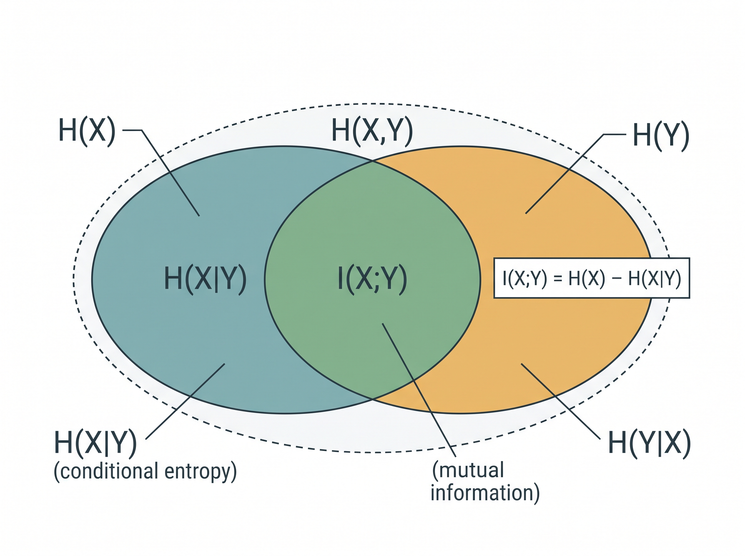
Mutual information is the reduction in entropy about one variable from observing another: $I(X;Y) = H(X) - H(X \mid Y)$. Read it as a before-and-after ledger. $H(X)$ is your doubt about the world state before the measurement; $H(X \mid Y)$ is your expected doubt after seeing sensor reading $Y$; the difference is what the measurement bought you, in bits. It is symmetric, $I(X;Y) = I(Y;X)$, and it is exactly $D_{\mathrm{KL}}\!\big(p(x,y)\,\|\,p(x)p(y)\big)$, the divergence between the joint and the product of marginals (the marginals being each variable's own standalone distribution, $p(x)$ and $p(y)$). So mutual information is zero if and only if $X$ and $Y$ are independent, meaning a sensor that carries no mutual information with the quantity you care about is, formally, useless for estimating it. The Mutual information section just below develops this quantity in full; the preview here sits alongside KL divergence because mutual information is itself a KL divergence, as the identity above shows.

Mutual information: the value of a measurement

Where cross-entropy priced the cost of trusting a wrong model, mutual information prices the payoff of a good measurement. That is the quantity a sensing engineer wants: it values a reading before you pay for it. Figure 4.5.1 lays out that payoff as a before-and-after ledger: the doubt you hold before the reading, minus the doubt left after it. Written through the joint distribution, the same quantity reads

Figure 4.5.1: Mutual information as a before-and-after entropy ledger. The left bar is the prior doubt H(X) about the hidden state; after observing sensor reading Y, the doubt shrinks to the residual H(X|Y). The green slice the measurement removes is the mutual information I(X;Y), the bits the reading bought you.

$$I(X;Y) = \sum_{x,y} p(x,y)\,\log_2 \frac{p(x,y)}{p(x)\,p(y)}.$$

It is the workhorse behind three recurring jobs. Feature selection: rank candidate features by their mutual information with the label and keep the informative ones, the information-theoretic backbone of Chapter 8. Sensor and channel selection: prefer the modality whose reading shares the most bits with the hidden state, and drop redundant sensors whose information is already covered, a principle that reappears in the fusion chapters of Part X. Representation learning: modern self-supervised objectives such as InfoNCE are, at heart, tractable lower bounds on mutual information between different views of a signal, as Chapter 17 develops. One caveat carries through all three: mutual information counts statistical dependence, not causation and not usefulness for a specific downstream cost. A feature can be richly informative and still awkward to act on. Treat it as a strong prior on value, not a verdict. Figure 4.5.2 illustrates mutual information as overlapping entropy circles (H(X), H(Y), H(X|Y), H(Y|X), joint entropy).

Mutual information as overlapping entropy circles (H(X), H(Y), H(X|Y), H(Y|X), joint entropy) — Figure 4.5.2: The entropy Venn diagram, showing how the joint entropy H(X,Y) decomposes into the two conditional entropies H(X|Y) and H(Y|X) and the shared mutual information I(X;Y) at their overlap.

Mental Model

Think of mutual information as a game of twenty questions about a mystery word. Before any question, your uncertainty is the entropy of the word; a well-chosen question is one whose answer you cannot predict, and hearing that answer slices the space of possible words roughly in half, buying you about one bit. Mutual information is exactly the average number of bits a given question's answer is expected to shave off your uncertainty: a question whose answer you could already guess, or that has nothing to do with the word, buys zero bits, just as a sensor statistically independent of the state carries zero mutual information with it. The point of picking a good sensor is the same as picking a good question, spend your one glance where the answer is both unknown and tied to what you want to know.

Common Misconception

A frequent error is the belief that zero correlation means two variables share no information, so an uncorrelated sensor can be safely discarded. Correlation only detects linear association, whereas mutual information captures any statistical dependence at all. A reading tied to the state by a symmetric or U-shaped rule, such as a magnitude that grows as the state moves away from center in either direction, can have exactly zero correlation yet substantial mutual information, and rejecting it on a correlation test throws away real bits.

Practical Example: The Robot That Priced Its Next Glance

A warehouse robot must decide whether a shelf bin is empty, half-full, or full before it plans a grasp. It carries three sensors it can poll: a cheap downward proximity sensor, a wrist camera it must rotate to aim (costing a second of motion), and a load cell in the gripper that requires an exploratory touch. Rather than firing all three, its planner estimates the mutual information $I(\text{bin state};\text{reading})$ for each from a small calibration log. The proximity sensor turns out to share only about 0.2 bits with the three-way state (it confuses half-full and full), the camera shares roughly 1.4 bits, and the touch shares 0.9 bits but is slow. The robot picks the camera first because it buys the most doubt-reduction per glance, and only falls back to touch when the camera's posterior entropy (the doubt still left in its belief after the reading) stays high (a glare-blinded frame). Before adopting this ledger the team had hand-tuned a fixed sensor order that wasted motion on the near-useless proximity ping. Pricing each measurement in bits turned a brittle heuristic into a rule that adapts per bin.

Step-Through: Pricing a Binary Sensor in Bits

Trace the mutual information ledger with a tiny $2 \times 2$ example: a hidden state $X$ (target present or absent, equally likely) and a binary sensor $Y$ that is right most of the time. Suppose the joint probabilities are $p(\text{absent},\text{low})=0.40$, $p(\text{absent},\text{high})=0.10$, $p(\text{present},\text{low})=0.10$, $p(\text{present},\text{high})=0.40$.

Step 1, marginals. $p(X)=(0.5, 0.5)$ and $p(Y)=(0.5, 0.5)$, so before measuring, $H(X) = -(0.5\log_2 0.5 + 0.5\log_2 0.5) = 1.000$ bit of doubt.

Step 2, score each cell by $p(x,y)\log_2\frac{p(x,y)}{p(x)p(y)}$. The matching cells have ratio $\frac{0.40}{0.25}=1.6$: each contributes $0.40 \times \log_2 1.6 = 0.40 \times 0.678 = 0.2712$. The mismatched cells have ratio $\frac{0.10}{0.25}=0.4$: each contributes $0.10 \times \log_2 0.4 = 0.10 \times (-1.322) = -0.1322$.

Step 3, sum the four cells. $I(X;Y) = 2(0.2712) + 2(-0.1322) = 0.5424 - 0.2644 = 0.278$ bit.

Step 4, read the ledger. The reading is expected to erase $0.278$ of your $1.000$ bit, leaving $H(X\mid Y) = 1.000 - 0.278 = 0.722$ bit of residual doubt. An 80-percent-accurate binary sensor buys you barely a quarter of the way to certainty, a sobering number that only mutual information makes visible.

The code below computes entropy and mutual information from a small joint sample, the exact calculation the robot's planner runs over its calibration log. It uses base-2 logs so the answers read directly in bits.

import numpy as np

def entropy(counts):
    p = counts / counts.sum()
    p = p[p > 0]                       # 0*log0 = 0
    return -np.sum(p * np.log2(p))     # bits

def mutual_information(joint):
    joint = joint / joint.sum()
    px = joint.sum(axis=1, keepdims=True)
    py = joint.sum(axis=0, keepdims=True)
    nz = joint > 0
    return np.sum(joint[nz] * np.log2(joint[nz] / (px @ py)[nz]))

# rows = hidden bin state (empty/half/full), cols = camera reading (low/mid/high)
joint = np.array([[40,  5,  1],
                  [ 6, 30,  8],
                  [ 1,  7, 42]], dtype=float)

print("H(state)      =", round(entropy(joint.sum(axis=1)), 3), "bits")
print("I(state;cam)  =", round(mutual_information(joint), 3), "bits")
# H(state) ~ 1.58 bits of prior doubt; the camera removes ~0.9 of them.

Estimating entropy and mutual information from a joint count table. H(state) is the robot's prior doubt about the bin (near the 1.585-bit maximum of a three-way choice); I(state;cam) is how many of those bits one camera reading is expected to remove. Ranking candidate sensors by this second number is the whole of information-driven sensor selection.

Right Tool: Skip the Estimator Plumbing

The hand-rolled functions above are fine for discrete tables, but real sensor readings are continuous, and estimating mutual information from continuous samples needs binning or nearest-neighbor tricks that are easy to get subtly wrong. scipy.stats.entropy gives entropy and KL divergence in one call, and scikit-learn's mutual_info_classif and mutual_info_regression estimate feature-label mutual information directly from raw continuous data using a validated k-nearest-neighbor estimator. That collapses a careful 60-to-80-line binning-and-bias-correction implementation into a single line, roughly a 95 percent reduction, while handling the continuous-variable bias that trips up naive histograms.

Real-World Application: Multimodal Medical Image Registration

When a hospital aligns a patient's computed tomography (CT) scan with a magnetic resonance imaging (MRI) scan so a surgeon sees both in one frame, the standard alignment criterion is mutual information: slide and rotate one image until the mutual information between the two intensity fields is maximized, because at perfect alignment each modality is maximally predictive of the other. This intensity-based scheme (Maes et al., 1997) is baked into the open-source ITK and Elastix toolkits that drive clinical and research registration pipelines. It works precisely because CT and MRI intensities are related nonlinearly, so a correlation-based aligner typically fails where mutual information succeeds.

Research Frontier

The k-nearest-neighbor estimators these libraries lean on quietly break down in high dimensions and on heavy-tailed sensor data. The NeurIPS 2023 benchmark Beyond Normal: On the Evaluation of Mutual Information Estimators (Czyz et al.) assembled a suite of distributions with known ground-truth mutual information and showed that classical estimators are badly biased once you leave the near-Gaussian regime. Diffusion-based neural estimators such as MINDE (Franzese et al., ICLR 2024) push past that ceiling, estimating mutual information for high-dimensional continuous signals in exactly the setting where the k-NN plumbing above would silently mislead you. For multimodal sensor fusion, where the hidden state couples to images, audio, and inertial streams at once, these estimators are how the "how many bits does this modality add" question is beginning to get an honest answer.

Information gain and deciding what to measure next

The payoff of this section is active sensing: choosing the next measurement that maximizes expected information gain. Suppose your current belief about a state $X$ has entropy $H(X)$, and a candidate action $a$ would yield an observation $Y_a$. The expected reduction in doubt is then the mutual information $I(X; Y_a)$ under that belief. Greedily picking $\arg\max_a I(X; Y_a)$ sits at the information-theoretic core of Bayesian experimental design, active learning (label the points that shrink model entropy the most), and next-best-view planning in robotics. It is also the quantitative version of the epistemic-uncertainty story from Section 4.4. High epistemic uncertainty means high entropy that data can remove, and mutual information tells you which datum removes the most. When you reach the Bayesian filters of Chapter 9 and the fusion rules of Part X, this same ledger decides which sensor to trust and when a reading is redundant. Bits, once you can count them, become a budget you can spend wisely.

Try It: Rank Real Features by Bits

Reproduce the sensor-selection ledger on a real multi-feature dataset in about fifteen minutes with a laptop and scikit-learn.

Load a labeled dataset: from sklearn.datasets import load_wine; X, y = load_wine(return_X_y=True). Treat its 13 continuous features as 13 candidate sensors and the 3-class label as the hidden state.
Estimate each feature's mutual information with the label: from sklearn.feature_selection import mutual_info_classif; mi = mutual_info_classif(X, y, random_state=0).
Sort and print the features in descending order of mi; note that a handful carry most of the bits while several carry almost none.
Train a LogisticRegression on only the top-3 features, then on all 13, and compare cross-validated accuracy to see how little the near-zero-MI features actually add.
Shuffle one high-MI feature with np.random.permutation and rerun step 2; confirm its mutual information collapses toward zero, since shuffling destroys the very dependence MI measures.

Lab: How Many Bits Survive the Noise?

Goal. Confirm empirically the theory that a noisier channel carries fewer bits, by watching the mutual information between a hidden signal and its noisy reading fall as you crank up the noise, and comparing it against the closed-form Gaussian-channel value for the signal-to-noise ratio (SNR), $I = \tfrac{1}{2}\log_2(1 + \mathrm{SNR})$.

Tools. Python with numpy and scikit-learn (sklearn.feature_selection.mutual_info_regression). No GPU, about 20 minutes.

Build it. Draw a hidden signal $x \sim \mathcal{N}(0,1)$ with 5000 samples. Simulate a sensor reading $y = x + \sigma\,\varepsilon$ with $\varepsilon \sim \mathcal{N}(0,1)$. Estimate $I(x;y)$ with mutual_info_regression(y.reshape(-1,1), x) and convert from nats to bits by dividing by $\ln 2$.

What to vary. Sweep the noise level $\sigma$ across, say, $\{0.1, 0.25, 0.5, 1, 2, 4\}$, which sweeps the SNR $\mathrm{SNR} = 1/\sigma^2$ over three orders of magnitude.

What to observe. Plot the estimated bits against $\log_{10}\sigma$ and overlay the theoretical curve $\tfrac{1}{2}\log_2(1 + 1/\sigma^2)$. You should see the estimate track the theory closely at low noise and both collapse toward zero bits as $\sigma$ grows: a channel drowning in noise transmits nothing, exactly as the entropy story predicts. As a stretch, replace the additive Gaussian noise with a squaring nonlinearity $y = x^2 + \sigma\varepsilon$ and confirm the k-NN estimator still reports positive bits even though the Pearson correlation between $x$ and $y$ is near zero.

Exercise

(a) A binary sensor fires with the correct label 80 percent of the time and is wrong 20 percent, independent of a uniform prior over two equally likely states. Compute $H(X)$, $H(X \mid Y)$, and $I(X;Y)$ in bits, and interpret the gap. (b) You are offered a second sensor whose reading is a perfect copy of the first. What is the mutual information of the pair with the state, and what does that tell you about paying for redundant sensors? (c) Using the code in this section, modify the joint table so the camera becomes useless (zero mutual information) without changing the marginal over states, and verify numerically.

Self-Check

Why is KL divergence not a valid distance metric, and what practical failure occurs when a model assigns zero probability to an event that actually happens?
State mutual information as an entropy difference and as a KL divergence between joint and product-of-marginals, and explain why both must give the same number.
Your feature has high mutual information with the label but adds nothing to a model that already uses a correlated feature. Which information-theoretic quantity captures that redundancy, and why is raw mutual information alone the wrong ranking?

What's Next

In Section 4.6, we turn the doubt-in-bits view into decisions with consequences: hypothesis testing and detection theory. Where mutual information asks how much a measurement could tell you, detection theory asks where to put the threshold once the reading arrives, trading false alarms against missed detections. The likelihood ratio you will meet there is the same log-probability machinery you just used to price surprise, now aimed at saying yes or no.