Hypothesis testing and detection theory

"Every alarm I raise is a bet. A false alarm costs me credibility; a missed detection costs me everything. My whole job is choosing the exchange rate between those two before the signal arrives."

A Decisive AI Agent

This section builds directly on the likelihood functions of Section 4.2 and the posterior reasoning of Section 4.3; a detector is a likelihood comparison with a threshold. It also leans on the noise distributions from Section 4.1 and, for where that noise physically comes from, the measurement models of Chapter 2. The vocabulary here becomes the backbone of classical anomaly and change detection in Chapter 12 and of radar target detection in Chapter 44.

Two hypotheses and two ways to be wrong

Frame every detection as a contest between a null hypothesis \(H_0\) (nothing is there; only noise) and an alternative \(H_1\) (signal present). A decision rule partitions the space of possible observations into a "declare \(H_1\)" region and a "declare \(H_0\)" region. Because the observation is random, the rule can fail in two distinct ways, and the asymmetry between them is the whole game. A Type I error (false alarm) declares a signal when there is none; its probability is \(P_{\text{FA}} = P(\text{declare } H_1 \mid H_0)\), conventionally called \(\alpha\). A Type II error (miss) stays silent when the signal is real; its probability is \(P_{\text{M}} = P(\text{declare } H_0 \mid H_1) = \beta\). The complement of a miss is the quantity we actually want to maximize, the detection probability or power, \(P_{\text{D}} = 1 - \beta\).

These two error rates trade against each other along a single knob. Lower the threshold to catch more real signals and you inevitably admit more noise-only false alarms; raise it to silence the false alarms and you start missing real events. You cannot drive both to zero with a fixed amount of data. The engineering question is never "how do I eliminate errors" but "given that I must trade, which exchange rate do I want, and what rule achieves it most efficiently?" In short: a detector never abolishes error, it only sets the exchange rate you pay between crying wolf and missing the wolf. Figure 4.6.1 makes this concrete: it overlays the two hypothesis distributions and shows how a single threshold carves the observation axis into a false-alarm tail and a miss tail.

The likelihood-ratio test is optimal

Choose this rule badly and you either bury operators under false brake events and phantom alarms or let a real cardiac event slip past in silence; choose it well and the very same noisy measurement delivers the highest detection rate physically possible at whatever false-alarm cost you can afford. Which rule wins? The Neyman-Pearson lemma gives a clean and slightly surprising answer: to maximize detection probability for any fixed false-alarm rate \(\alpha\), compare the likelihood ratio to a threshold and nothing else. Given observation \(x\), form

where the threshold \(\eta\) is tuned so the false-alarm rate equals your budget \(\alpha\). No other test, however clever, achieves higher power at that \(\alpha\). The threshold need not come from a false-alarm budget at all: when you instead know the prior probabilities of the two hypotheses and the cost of each kind of error, the same ratio is compared against a threshold set by the cost ratio times the prior odds, which is the Bayes (minimum-risk) rule that Exercise (c) asks you to derive. This is a strong optimality result: the entire high-dimensional observation collapses to one sufficient statistic (a single number that carries every bit of the data relevant to choosing between the two hypotheses, so nothing is lost by discarding the rest), the ratio, and the only free choice left is where to cut it. When the two hypotheses are Gaussian with the same covariance, taking the logarithm turns the ratio into a linear function of \(x\) (the logarithm is monotonic, so comparing \(\log\Lambda(x)\) to a threshold decides exactly the same cases as comparing \(\Lambda(x)\), just in a simpler algebraic form), which is why the classical matched filter (correlate the incoming signal with a template, then threshold) is the optimal detector for a known waveform in white Gaussian noise. Detecting a chirp in radar, a QRS complex in an electrocardiogram (ECG), or a known vibration signature in a bearing all reduce to the same correlate-and-threshold skeleton.

For a known signal of energy \(E\) in white noise of power spectral density \(N_0/2\), the achievable performance depends only on the ratio \(d^2 = 2E/N_0\), the deflection or effective signal-to-noise ratio (SNR). Larger \(d\) pushes the two hypothesis distributions apart and lets you get both low \(\alpha\) and high \(P_{\text{D}}\); that single scalar summarizes how detectable the signal fundamentally is, independent of the threshold you later pick. Yet that lone number says nothing about which threshold is worth choosing, so to expose the full menu of operating points we sweep the threshold and plot the detector's entire trade-off curve.

ROC curves: reading a detector's whole character

Sweep the threshold across its full range and plot \(P_{\text{D}}\) against \(P_{\text{FA}}\), and you trace the Receiver Operating Characteristic (ROC) curve, an idea that literally comes from World War II radar operators. The curve rises from \((0,0)\), where the threshold is so high nothing is ever declared, to \((1,1)\), where everything is. A useless detector that ignores the data sits on the diagonal; a perfect one hugs the top-left corner. The area under the curve (AUC) compresses the whole picture into one number: the probability that the detector ranks a random true event above a random noise sample. The curve itself is what you deploy against, because the right operating point depends on the relative cost of a false alarm versus a miss in your application. The code below builds an ROC from scratch for a Gaussian detection problem. Figure 4.6.2 illustrates ROC curve construction from threshold sweep.

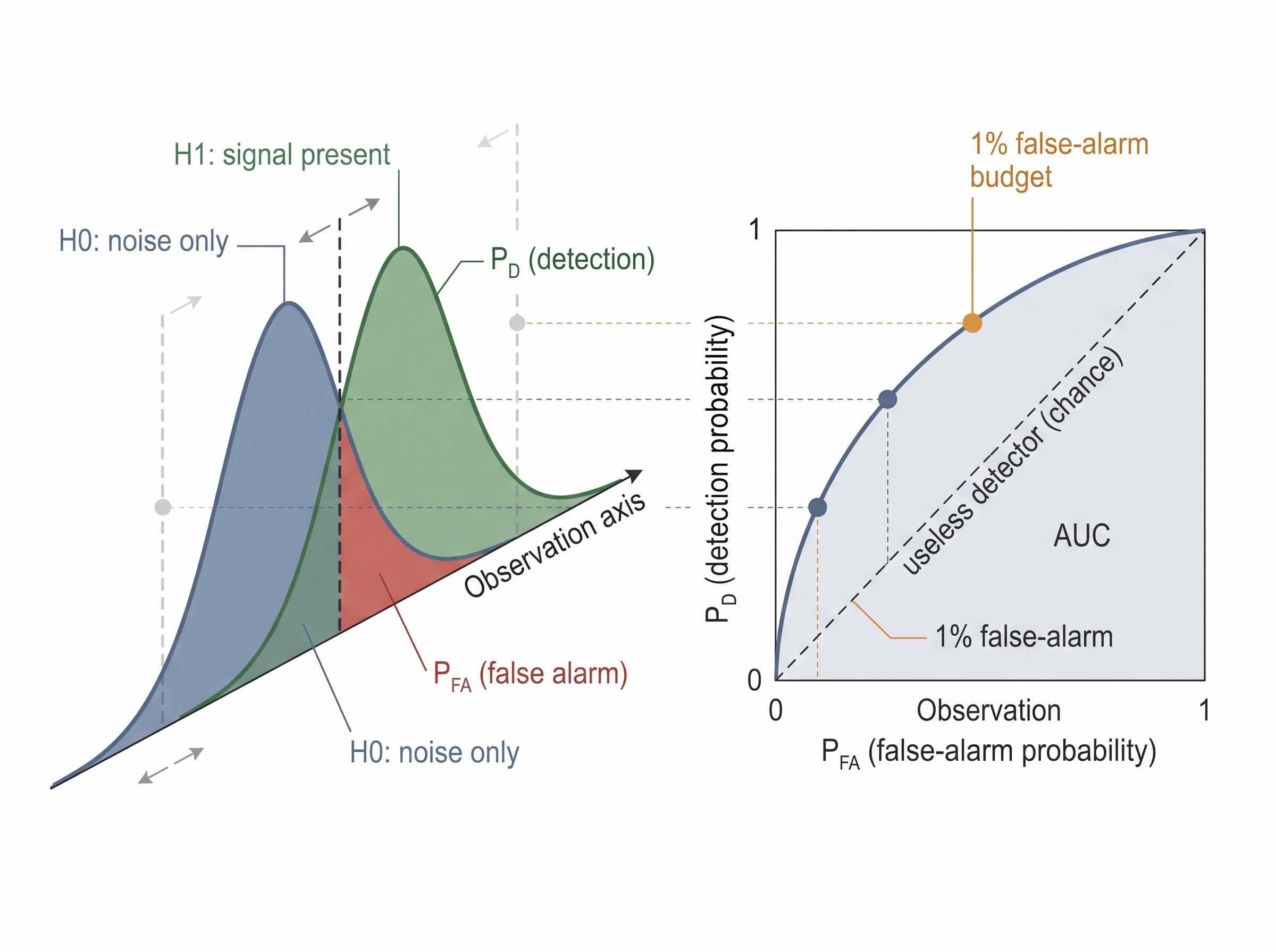
The area under the curve deserves a precise reading of its own. Concretely, AUC is the probability that the detector assigns a higher score to a randomly drawn true event than to a randomly drawn noise sample, so 0.5 is coin-flip-useless and 1.0 is perfect separation. It matters because it collapses ranking quality across every possible threshold into one number, which lets you compare two detectors before committing to any operating point; it earns that summary by integrating \(P_{\text{D}}\) over all \(P_{\text{FA}}\) values as the threshold sweeps. Reach for AUC when you want a single threshold-free score to screen or rank candidate detectors, but switch back to a specific point on the ROC (or to a precision-recall curve) the moment you deploy, since deployment fixes exactly one threshold and rare-event costs can make whole regions of the curve irrelevant.

import numpy as np

def roc_from_scores(scores, labels, n_points=200):
    # scores: detector statistic (e.g. log-likelihood ratio); labels: 1=signal, 0=noise
    thr = np.linspace(scores.min(), scores.max(), n_points)
    P = labels.sum(); N = (labels == 0).sum()
    pfa, pd = [], []
    for t in thr:
        fire = scores >= t
        pd.append(np.sum(fire & (labels == 1)) / P)   # detection prob
        pfa.append(np.sum(fire & (labels == 0)) / N)  # false-alarm prob
    pfa, pd = np.array(pfa), np.array(pd)
    auc = np.trapz(pd[::-1], pfa[::-1])               # integrate along PFA
    return pfa, pd, auc

rng = np.random.default_rng(0)
d = 2.0                                               # deflection (signal separation)
noise  = rng.normal(0.0, 1.0, 20000)                 # H0 samples
signal = rng.normal(d,   1.0, 20000)                 # H1 samples
scores = np.concatenate([noise, signal])
labels = np.concatenate([np.zeros(20000), np.ones(20000)])
pfa, pd, auc = roc_from_scores(scores, labels)
print(f"AUC = {auc:.3f}")                             # ~0.921 for d = 2
# operating point closest to a 1% false-alarm budget:
i = np.argmin(np.abs(pfa - 0.01))
print(f"at PFA={pfa[i]:.3f}, detection prob PD={pd[i]:.3f}")

The last two lines refuse a single accuracy figure: they pin the operating point to a false-alarm budget, then read off the detection probability bought at that price. That is the honest way to quote a detector, and the discipline Chapter 65 demands for leakage-safe benchmarking.

Deciding over time, and the peril of many tests

Adapting the threshold across neighboring cells in space, as CFAR does, is only half the story, because a sensor stream also forces us to decide as evidence unfolds over time. Two extensions matter constantly in streaming sensor systems. First, you rarely get one shot. If samples keep arriving, Wald's sequential probability ratio test (SPRT) accumulates the log-likelihood ratio. It declares the moment that running total crosses an upper bound (signal) or lower bound (noise), and otherwise waits for more data. For the same error rates, sequential testing reaches a decision with fewer samples on average than any fixed-sample test. That efficiency is why it underlies low-power wake-word and change-point detectors: decide early on easy cases, and keep listening only when the evidence is genuinely ambiguous. Change detection in Chapter 12 builds its cumulative sum (CUSUM) algorithm directly on this accumulating-evidence idea.

Second, beware the multiplicity trap. A monitoring system that runs one test per second at a one-percent false-alarm rate produces, in expectation, 36 false alarms every hour purely by chance, with the data behaving exactly as it should. A p-value is the probability, under \(H_0\), of a statistic at least as extreme as observed; it is not the probability that \(H_0\) is true, and it is not a measure of effect size. Because that p-value is uniform under \(H_0\), enough tests will always surface small ones. When you test many hypotheses, control the family-wide error (a Bonferroni cap on \(\alpha\), or a false-discovery-rate (FDR) procedure) rather than each test in isolation. Sensor fleets that ignore this drown their operators in spurious alerts and train them to ignore the real ones.

What's Next

Section 4.7 turns to Monte Carlo and sampling, the workhorse for the many detection and estimation integrals that have no closed form. When the likelihood ratio, the false-alarm rate, or the threshold cannot be computed analytically, we estimate them by drawing samples, and the same sampling machinery will later power the particle filters and Bayesian computations that recur throughout the book.