Monte Carlo and sampling basics

"When I cannot solve the integral, I ask ten thousand dice to vote on the answer, and I trust the average of their opinions."

A Statistically Enfranchised AI Agent

This section assumes the random variables, distributions, and expectations of Chapter 4, sections 4.1 through 4.3, and it uses the aleatoric-versus-epistemic distinction of section 4.4 to decide what to sample. Section 2 of Chapter 2 supplies the noise models behind these distributions if you have not met them. It needs no measure theory; the law of large numbers is enough.

The Monte Carlo estimator: averaging your way to an integral

Every uncertainty number a sensor system reports, every confidence interval on a fault probability, every particle-filter update ultimately rests on the one estimator below. Get its convergence wrong and a device ships a reliability guarantee it cannot keep. What. Monte Carlo estimation answers the question "what is \(\mathbb{E}_{x\sim p}[f(x)]\)?" by drawing \(N\) independent samples \(x_1,\dots,x_N\) from \(p\) and computing the sample mean

Why it works. The estimator \(\hat{\mu}_N\) is unbiased: its expectation equals the true integral for every \(N\). By the law of large numbers it converges to the true value as \(N\) grows. The central limit theorem (the result that a sum of many independent contributions tends toward a Gaussian shape) then makes its error approximately Gaussian with standard deviation \(\sigma/\sqrt{N}\), where \(\sigma^2 = \operatorname{Var}_p[f(x)]\). That \(\sqrt{N}\) is the single most important fact in this section. To halve your error you must quadruple your samples. The error does not care how many dimensions \(x\) has, which is why Monte Carlo typically beats grid-based numerical integration once your state vector grows past roughly three or four dimensions. A 12-dimensional inertial measurement unit (IMU) plus bias state would need a grid of astronomical size; the same accuracy from Monte Carlo needs only enough samples to tame the variance.

How you use it. Nearly every quantity you want is an expectation in disguise. A probability \(P(A)\) is \(\mathbb{E}[\mathbb{1}_A]\), the expected value of an indicator. A quantile is found by sampling and sorting. A predictive mean is \(\mathbb{E}[f(x)]\); a predictive variance is \(\mathbb{E}[f(x)^2]-\mathbb{E}[f(x)]^2\). Choose \(f\), draw from \(p\), average. In short: Monte Carlo turns any question you can phrase as an expectation into three verbs, sample, evaluate, average. The pipeline in Figure 4.7.1 traces those three verbs end to end, from the target distribution to an estimate carrying its own error bar.

Turning uniform noise into any distribution

What. The estimator of the previous subsection took for granted that you could already draw samples from \(p\); producing those draws is the problem we solve now. Your hardware random-number generator gives you one primitive: uniform draws on \([0,1)\). Everything else is built from that primitive by transformation.

How, method one: inverse transform. If \(F\) is the cumulative distribution function (CDF) of a scalar random variable and \(U\sim\text{Uniform}(0,1)\), then \(X = F^{-1}(U)\) has exactly the distribution you wanted. This is why an exponential inter-arrival time for a Poisson event stream is generated as \(-\lambda^{-1}\ln(1-U)\): the log is the inverse CDF. Inverse transform is exact and cheap whenever you can invert \(F\).

How, method two: rejection sampling. When you cannot invert \(F\) but you can evaluate an unnormalized density \(\tilde{p}(x)\) (a density you can compute only up to an unknown overall constant, the usual situation for a Bayesian posterior), wrap it in a proposal \(q(x)\) you can sample, scaled so that \(M\,q(x)\ge\tilde{p}(x)\) everywhere. Draw \(x\sim q\), accept it with probability \(\tilde{p}(x)/(M\,q(x))\), and repeat. Accepted samples are distributed exactly as \(p\). The catch is efficiency: the acceptance rate is \(1/M\), so a loose envelope in high dimensions wastes almost every draw.

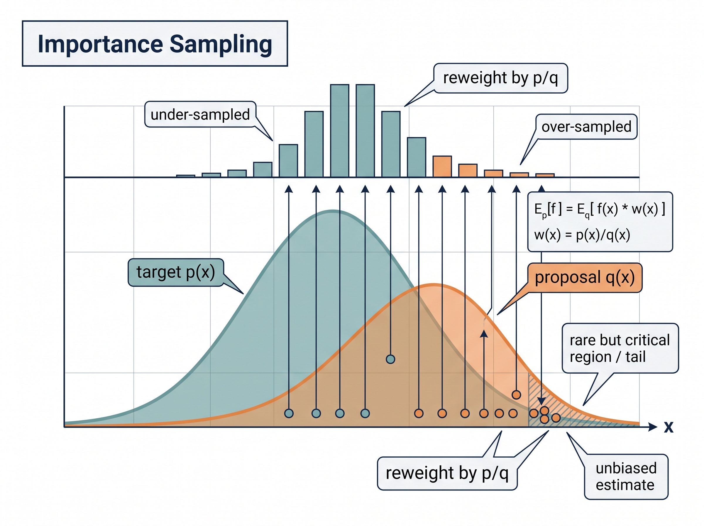
How, method three: importance sampling. Sometimes you cannot or should not draw from \(p\) at all. Instead draw from a convenient \(q\) and reweight: \(\mathbb{E}_p[f] = \mathbb{E}_q[f(x)\,w(x)]\) with weights \(w(x)=p(x)/q(x)\). This is the mathematical heart of the particle filter you will build in Chapter 10, where \(q\) is the motion model and the weights carry the measurement likelihood. Importance sampling shines when you deliberately over-sample a rare but critical region, such as the tail where a fall-detection alarm should fire. You then correct the bias with the weights. Figure 4.7.2 illustrates importance sampling reweighting.

How many samples? Error bars on your error bars

What. Now that you can generate and reweight samples by any of the three methods above, the next question is how far to trust the average they produce. A Monte Carlo estimate without an uncertainty is half an answer. Because \(\hat{\mu}_N\) is itself a random variable, you can estimate its standard error from the very same samples: \(\widehat{\text{SE}} = \hat{\sigma}/\sqrt{N}\), where \(\hat{\sigma}\) is the sample standard deviation of the \(f(x_i)\) values. Report \(\hat{\mu}_N \pm 1.96\,\widehat{\text{SE}}\) for an approximate 95% interval.

Why it matters for sensing. When you estimate a rare-event probability such as a \(10^{-4}\) false-alarm rate, naive sampling needs on the order of \(10^6\) draws just to see a handful of events, and the relative error stays enormous until you do. This is exactly where importance sampling earns its keep: bias the proposal toward the tail, and with a well-matched proposal the same accuracy can arrive with orders of magnitude fewer draws. The estimator that turns raw draws into an answer with a defensible interval is the code below.

import numpy as np

rng = np.random.default_rng(42)

def mc_estimate(f, sampler, n, batch=100_000):
    """Streaming Monte Carlo mean with a 95% standard-error interval.
    Batches keep memory flat, which matters on edge hardware."""
    total, total_sq, count = 0.0, 0.0, 0
    while count < n:
        m = min(batch, n - count)
        vals = f(sampler(m))          # f applied to a batch of draws
        total    += vals.sum()
        total_sq += (vals ** 2).sum()
        count    += m
    mean = total / count
    var  = total_sq / count - mean ** 2
    se   = np.sqrt(max(var, 0.0) / count)
    return mean, 1.96 * se

# Estimate P(||accel bias|| > 0.05 g) for a 3-axis IMU with correlated bias.
cov = np.array([[4e-4, 1e-4, 0.0],
                [1e-4, 4e-4, 0.0],
                [0.0,  0.0,  9e-4]])   # units of g^2
L = np.linalg.cholesky(cov)
sample_bias = lambda m: (L @ rng.standard_normal((3, m))).T
exceeds = lambda b: (np.linalg.norm(b, axis=1) > 0.05).astype(float)

p_hat, halfwidth = mc_estimate(exceeds, sample_bias, n=2_000_000)
print(f"P(exceed) = {p_hat:.4f} +/- {halfwidth:.4f}")

The example applies the estimator to a real specification question: how often does an IMU's correlated bias vector exceed a magnitude limit? The Cholesky factor, a lower-triangular matrix \(L\) that acts as a matrix square root of the covariance so that \(LL^{\top}=\Sigma\), turns independent Gaussian draws into correlated ones, a trick you will reuse constantly when the noise channels of a sensor are coupled. The returned half-width tells you whether two million samples were enough or whether you should keep drawing.

Variance reduction and low-discrepancy sampling

What. Since error scales as \(\sigma/\sqrt{N}\) and buying more \(N\) is expensive on an edge device, the smart move is to shrink \(\sigma\). Three techniques recur throughout sensing.

Variance reduction is precisely the practice of replacing your estimator with a different, still-unbiased estimator of the same quantity that has smaller variance, so each sample buys more accuracy. It matters because the \(\sigma/\sqrt{N}\) law makes brute-force accuracy quadratically expensive: cutting \(\sigma\) in half is worth as much as quadrupling \(N\), and it costs no extra draws. Mechanically, every method here rewrites the target expectation so that the random part you actually average has less spread, whether by pairing draws that cancel, subtracting a known-mean term, or forcing even coverage. Reach for variance reduction whenever samples are expensive or the integrand has exploitable structure; stick with plain sampling when draws are cheap and you value the simple, independent error bars.

Antithetic variates. For every draw \(x\), also use its mirror image (for a symmetric distribution, \(-x\) after centering). Positively correlated errors cancel, and a symmetric integrand can see its variance drop sharply at zero extra sampling cost. Control variates subtract a correlated quantity whose expectation you know analytically, replacing part of the noisy estimate with an exact term. Stratified sampling partitions the domain and samples each stratum in proportion, guaranteeing coverage rather than trusting luck.

Quasi-Monte Carlo. Instead of pseudo-random points, use a deterministic low-discrepancy sequence such as Sobol or Halton that fills space more evenly than random draws ever do. For smooth integrands the error can improve toward \(1/N\) rather than \(1/\sqrt{N}\), a decisive speedup. At a million samples that is, in the best case of a sufficiently smooth integrand, the gap between an error near \(10^{-3}\) and one near \(10^{-6}\), a thousandfold sharper answer for the same budget. This is the workhorse behind the digital-twin and synthetic-data sweeps of Chapter 55, where you want to cover a parameter space of sensor placements or lighting conditions without wasting simulation budget on clumped points. As of 2024, you rarely code these sequences by hand: scipy.stats.qmc (added in SciPy 1.7, 2021) supplies Sobol and Halton generators with proper scrambling and balance checks, and has largely replaced hand-rolled low-discrepancy code.

When to reach for each. Use antithetic and control variates when you have structure you can exploit and evaluations are cheap. Use quasi-Monte Carlo for smooth, moderate-dimensional integrals such as calibration sweeps. Fall back to plain pseudo-random sampling when the integrand is rough, discontinuous, or when you need the honest, well-understood \(\sqrt{N}\) error bars that the central limit theorem guarantees; low-discrepancy sequences complicate confidence-interval construction because their points are not independent.

What's Next

Chapter 5 leaves the world of clean synthetic draws and confronts real recorded data: how to build datasets from sensor streams without leaking future information into the past, how to split by device and by time rather than at random, and how the sampling intuition from this section informs honest train-test protocols. The same law of large numbers that made these estimators trustworthy also warns what happens when samples are correlated rather than the independent draws Monte Carlo assumed.