Section 2.7: Measurement models as the bridge to AI

"They kept asking me to predict the future. I kept explaining that I had never once been told what the present actually was, only what a sensor felt like saying about it."
A Pedantic AI Agent

The big picture

Everything in this chapter has been a defect: the wrong observable (Section 2.1), a coarse or clipped scale (Sections 2.2 and 2.4), noise (Section 2.3), a lagging transfer function (Section 2.5), a crowd of environmental couplings (Section 2.6). This closing section does one thing: it gathers all of them into a single object, the measurement model, a function that maps the true state of the world $x$ to the number a sensor emits $y$. Writing that map down is the pivot on which the rest of the book turns. Once you have $y = h(x) + \text{noise}$, you can run it forward to simulate, invert it to estimate, turn it into a likelihood to fuse, or hand its residual to a network to learn. A measurement model is not bookkeeping about a broken sensor. It is the interface contract between physics and every AI method that follows: estimation, filtering, anomaly detection, and the learned models of Parts IV and V. This is the bridge, and the traffic on it goes both ways.

This section assumes the whole of Chapter 2: the observables of Section 2.1, the transfer function of Section 2.5, and the coupled, multivariable view of Section 2.6. It points forward to the probability and estimation machinery of Chapter 4, which formalizes the likelihood we build here, and to Chapter 9, where the measurement model becomes the observation equation of a Kalman filter.

The measurement model: one equation that eats the whole chapter

Ship a robot that takes a saturated, drifting reading at face value and it will steer with total confidence into a wall it can no longer perceive; the cure is not a better sensor but an honest account of how the sensor distorts the world. That account is the measurement model, and it is the one object this whole section is built to earn. A measurement model, sometimes called a forward model or observation model, is the map from latent state (the hidden true condition of the world you cannot observe directly) to observed reading. In its general stochastic form,

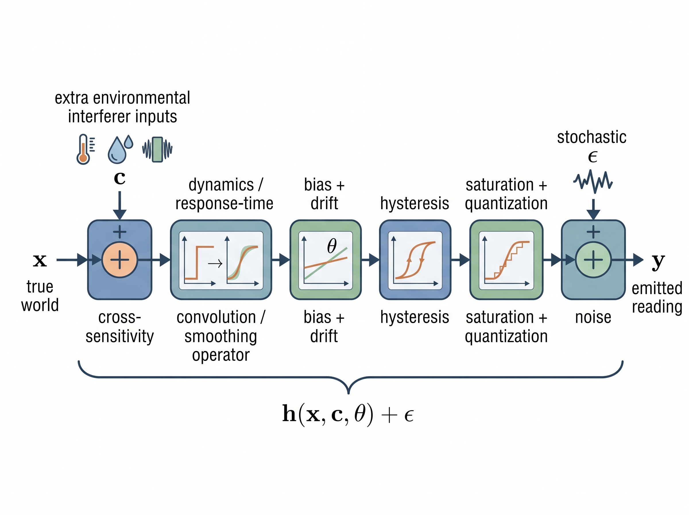
$$y_t = h(x_t,\; \mathbf{c}_t,\; \boldsymbol{\theta}) + \varepsilon_t, \qquad \varepsilon_t \sim p_\varepsilon,$$

where $x_t$ is the quantity you actually care about, $\mathbf{c}_t$ are the environmental interferers, $\boldsymbol{\theta}$ are (mostly per-device) calibration parameters, and $\varepsilon_t$ is the stochastic residual. Every pathology from this chapter is now a named piece of $h$. Finite resolution and saturation are a quantizing, clipping nonlinearity on the output. Bias and drift are slow terms in $\boldsymbol{\theta}$; hysteresis makes $h$ depend on the history of $x$, not just its current value. The transfer function and response time make $h$ a dynamical operator (a convolution), so $y_t$ is a smeared function of the recent trajectory of $x$. Cross-sensitivity is the dependence on $\mathbf{c}_t$. The noise lives in $p_\varepsilon$, and its color (Section 2.3) means $\varepsilon_t$ is generally not independent across time. One of the most useful habits in sensor AI is to keep this equation explicit rather than letting each defect leak into your pipeline as an unlabeled surprise. In short: write down how the sensor lies, or spend the rest of the pipeline being ambushed by it. Figure 2.7.2 illustrates the anatomy of the forward model h: every Chapter 2 defect as a named stage in the sensing pipeline.

Anatomy of the forward model h: every Chapter 2 defect as a named stage in the sensing pipeline — Figure 2.7.2: The forward model h decomposed into a pipeline of named stages, one per Chapter 2 defect, that together transform the true state x into the emitted reading y.

Common Misconception

A frequent mistake is to assume that writing $h$ down means you can algebraically invert it to recover $x$, that you just solve $y = h(x)$ for $x$. But most of the defects above make $h$ non-invertible: saturation discards every value beyond its clip, and the response-time convolution smears many different trajectories into the same reading, so no exact inverse exists. Recovering $x$ is therefore statistical estimation under uncertainty, not algebra, which is exactly why the rest of the book reaches for likelihoods and filters instead of a single solve step.

Key insight: the direction of the arrow is everything

The measurement model is written forward: world causes reading, $x \to y$. But at inference time you have $y$ and want $x$, which is the arrow reversed. That reversal is the central act of nearly every method in this book. Estimation, filtering, calibration, and inverse imaging all answer "given the reading and a model of how readings are produced, what state is most consistent with it?" The forward model is usually easy and physical; the inverse is usually hard, often ill-posed (many different states can produce the same reading, so the answer is not unique or is wildly sensitive to noise), and is where the intelligence goes. If you cannot write the forward model, you are guessing at the inverse. If you can, you have converted a vague perception problem into a well-defined inverse problem with known structure and a known noise budget.

Mental Model

Think of baking a cake. The recipe is the forward model: given the flour, sugar, eggs, and oven schedule, it tells you exactly what comes out, and running it forward is straightforward. Now hand someone a single finished slice and ask them to name the precise gram-weights and the oven curve that produced it. That is the inverse, and it is genuinely hard: many different ingredient sets bake into nearly identical slices, and a crumb of measurement noise (one slightly stale egg) can point you at the wrong recipe entirely. Estimation is this exact act of reading the slice to reconstruct the recipe, which is why the reversed arrow, not the forward one, is where the real work lives.

Three ways AI consumes a measurement model

Writing $h$ down pays off in three distinct modes, and most systems use more than one. Figure 2.7.1 lays out the shared skeleton: the forward map $h$ runs left to right from state to reading, and each of the three modes taps that same map at a different point.

Figure 2.7.1: The forward measurement model $h$ maps true state $x$ to reading $y$ (solid arrows); inference reverses that arrow (dashed). The three consumption modes attach to the same map: mode 1 runs it forward as a generator, mode 2 inverts it as an estimator through the likelihood, and mode 3 embeds it as inductive bias inside a learned model.

Forward, as a generator. Run $h$ on known states to synthesize realistic readings. This is how you build simulators, augment scarce data with physically valid corruptions, and stress-test a model against saturation or drift it has not seen in the field. Lab 2, below, is exactly this mode: inject bias, drift, saturation, and colored noise through the forward model and measure what they do downstream. Synthetic data and digital twins (live simulation models kept continuously in sync with a physical asset) in Chapter 55 scale this idea into a full engineering discipline.

Inverse, as an estimator. Given $y$, recover $x$. When $h$ is known and invertible, this is calibration and compensation. When $h$ is a dynamical, noisy operator, the principled inverse is Bayesian filtering: the measurement model becomes the likelihood $p(y_t \mid x_t)$, where the likelihood is the probability of seeing reading $y_t$ supposing the true state were $x_t$, a motion model supplies the prior $p(x_t \mid x_{t-1})$, and Bayes' rule fuses them. The Kalman family of Chapter 9 is precisely this pattern with $h$ linear and $p_\varepsilon$ Gaussian. The uncertainty propagation that makes the estimate trustworthy is the subject of Chapter 4.

As inductive bias, feeding a learned model. When $h$ is only partly known, you keep the part you trust and learn the rest. Feed the interferer channels $\mathbf{c}_t$ as explicit inputs so the network can learn the coupling it should undo; subtract the analytic forward prediction and let a model clean up the residual; or embed $h$ inside a differentiable pipeline so gradients flow through the physics (physics-informed learning). This hybrid stance, physics where you have it, learning where you do not, is the theme running from the deep models of Chapter 13 through the fusion methods of Part X. The third of those modes is common enough, and distinct enough, to have earned a name of its own.

Checkpoint

So far: a measurement model is consumed in three ways, run forward as a generator of synthetic data, inverted as an estimator through the likelihood, or embedded as inductive bias inside a learned model.

Physics-informed learning, named

The technique named here, physics-informed learning, is any method that constrains a learned model with a known piece of the forward physics instead of letting it discover everything from data. It matters because the physics you inject acts as free supervision: in practice it cuts the volume of labeled data you need and lets the model extrapolate along the governing equation rather than only interpolating inside the training cloud. Mechanically you do one of three things: feed the known interferers $\mathbf{c}_t$ as explicit inputs, learn only the residual left after subtracting the analytic prediction, or make $h$ a differentiable layer so training gradients flow through the physics. Reach for it when you trust part of the model but not all of it; prefer a purely analytic model when the physics is complete and a purely learned one when no usable equation exists at all.

Practical example: an automotive wheel-speed sensor that learned to disbelieve itself

A driver-assistance stack estimated vehicle speed from four Hall-effect wheel-speed sensors, where a Hall-effect sensor emits a voltage pulse each time a magnet on the rotating wheel passes a fixed pickup. Each sensor's measurement model was well understood: pulse count is proportional to wheel rotation, but the proportionality (the $\boldsymbol{\theta}$ tire circumference) drifts with tire wear, pressure, and temperature, and saturates into noise below a crawl. The team resisted the temptation to regress speed directly from raw pulses with a big network. Instead they wrote the forward model, made it the observation equation of a filter that fused the four wheels with the inertial measurement unit, and let the filter estimate the slowly-drifting per-wheel scale factors online as extra states. During a hard brake, one wheel locked and its reading went to zero; because the measurement model told the estimator that a single zero reading was wildly inconsistent with the other three wheels and the accelerometer, the filter down-weighted it automatically instead of believing the car had stopped. A model without the explicit measurement equation had no principled way to know which sensor to distrust. The orientation and dead-reckoning machinery this leans on is developed in Chapter 24.

From model to likelihood: the exact hinge to inference

The step that turns a measurement model into something an inference engine can use is to stop treating $h$ as producing a number and start treating it as producing a distribution. Rearranging the forward model, the probability of seeing reading $y$ if the state were $x$ is

$$p(y \mid x) = p_\varepsilon\big(y - h(x, \mathbf{c}, \boldsymbol{\theta})\big).$$

This likelihood is the single most reused object in the book. Maximizing it over $x$ gives the maximum-likelihood estimate; combining it with a prior gives the Bayesian posterior of Chapter 4; iterating it over time gives a filter. Crucially, the shape of $p_\varepsilon$ is not a detail. Suppose your noise is heavy-tailed because of occasional dropouts. A Gaussian likelihood then lets a single outlier drag your estimate anywhere, while a heavy-tailed likelihood makes the estimator robust for free. The measurement model is where you get to state plainly how your sensor lies, and that statement is what lets the estimator not be fooled. The small program below composes several chapter-2 defects into one forward model. It then recovers the state by maximizing the likelihood and contrasts that with a naive readout.

import numpy as np
from scipy.optimize import minimize_scalar

rng = np.random.default_rng(0)

# Forward measurement model h(x): gathers chapter-2 defects
S, bias, drift_rate, sat = 2.0, 0.5, 0.01, 8.0   # sensitivity, bias, drift, saturation
def h(x, t):
    y = S * x + bias + drift_rate * t             # sensitivity + bias + slow drift
    return np.clip(y, -sat, sat)                   # saturation nonlinearity

# Simulate one reading at time t with heavy-tailed (Student-t) noise
x_true, t = 2.3, 40.0
y_obs = h(x_true, t) + 0.4 * rng.standard_t(df=3)  # colored, heavy-tailed residual

# Naive inverse: invert only the nominal sensitivity
x_naive = y_obs / S

# Model-based inverse: maximize a robust likelihood of the FULL model
def neg_log_lik(x):                                # Student-t is outlier-tolerant
    r = (y_obs - h(x, t)) / 0.4
    return np.sum(np.log1p(r**2 / 3))
x_hat = minimize_scalar(neg_log_lik, bounds=(-10, 10), method="bounded").x

print(f"true x            : {x_true:.3f}")
print(f"naive readout     : {x_naive:.3f}")
print(f"model-based x_hat : {x_hat:.3f}")

Composing chapter-2 defects into one forward model h, then inverting it by maximizing a robust likelihood. The naive readout inherits the bias and drift wholesale; the model-based estimate, knowing exactly how the reading was produced, subtracts them and shrinks the gap to the true state. Fit and evaluate the calibration parameters on held-out conditions, never on the stream you will score.

The exact numbers are not the point. The naive readout cannot know about the bias or the drift; the model-based estimate can, because we handed it the forward map. That is a measurement model's whole value in one screen of Python.

Step-Through: inverting a saturating, biased sensor by maximizing the likelihood

Trace the inversion with concrete numbers. Fix the forward model $h(x) = \operatorname{clip}(2x + 0.5 + 0.01 t,\,-8,\,8)$ and read the sensor at time $t = 40$, so the drift term is $0.01 \times 40 = 0.4$ and $h(x) = \operatorname{clip}(2x + 0.9,\,-8,\,8)$. The true state is $x_{\text{true}} = 2.3$, so the noiseless reading is $h(2.3) = 2(2.3) + 0.9 = 5.5$; one draw of heavy-tailed noise adds $+0.2$, giving $y_{\text{obs}} = 5.7$.

Naive readout. Divide by the nominal sensitivity only: $x_{\text{naive}} = 5.7 / 2 = 2.85$. It has swallowed the whole $0.9$ of bias-plus-drift and lands $0.55$ above the truth.
Score candidate $x = 2.0$. Predict $h(2.0) = 4.9$; residual $r = (5.7 - 4.9)/0.4 = 2.0$; robust loss $\log(1 + r^2/3) = \log(1 + 1.333) = 0.847$.
Score candidate $x = 2.4$. Predict $h(2.4) = 5.7$; residual $r = 0$; loss $\log(1 + 0) = 0$. This is the minimum so far.
Score the naive guess $x = 2.85$. Predict $h(2.85) = 6.6$; residual $r = (5.7 - 6.6)/0.4 = -2.25$; loss $\log(1 + 5.06/3) = 0.988$, the worst of the three.
Read off the estimate. The optimizer settles at $\hat{x} \approx 2.4$, a gap of $0.1$ from the truth versus $0.55$ for the naive readout. Knowing that $0.9$ offset lived inside $h$ is exactly what let the estimator subtract it.

Library shortcut

Hand-rolling the likelihood, its gradient, and a robust optimizer is instructive once and tedious forever. When your measurement model is a linear-Gaussian observation equation, filterpy's KalmanFilter turns the whole forward-model-plus-inversion into kf.H = ...; kf.R = ...; kf.predict(); kf.update(y), roughly four lines replacing the fifty or more you would write for the predict/update covariance algebra by hand. For nonlinear or non-Gaussian $h$, probabilistic-programming tools such as NumPyro or Stan take your forward model as a few lines of generative code and hand back the full posterior over $x$ and $\boldsymbol{\theta}$, no manual gradient derivation required. You still supply the physics; the library supplies the inference calculus.

Research Frontier

This section inverts a measurement model by writing its likelihood explicitly, but a fast-moving line of work inverts $h$ even when the likelihood is intractable or the prior over $x$ is a rich natural signal. Diffusion Posterior Sampling (Chung et al., ICLR 2023) pairs a diffusion-model prior over plausible states with the known forward operator $h$ and its noise model, then samples the posterior $p(x \mid y)$ directly, cracking noisy nonlinear inverse problems (deblurring, inpainting, tomography) that no closed-form inverse can touch. More broadly, simulation-based inference toolkits such as sbi learn the posterior from forward-model simulations alone, so you supply only a runnable $h$ and never derive a likelihood by hand.

The measurement model that almost never got published, then flew to the Moon

When Rudolf Kalman circulated the idea that a measurement model could be written as an observation equation and inverted recursively, the reception was chilly. He later recounted that established control theorists were skeptical, and the work was steered away from the mathematics journals toward a mechanical-engineering one, where his 1960 paper finally landed. The vindication was spectacular: a few years later Stanley Schmidt at NASA Ames recognized that this exact forward-model-plus-inversion loop was what Apollo needed, and a version of the filter ran on the Apollo Guidance Computer, fusing star-sightings and accelerometer readings to navigate to the Moon in a machine with roughly four kilobytes of usable memory, less than a single modern JPEG thumbnail. The humble equation $y = h(x) + \text{noise}$ went from unpublishable to load-bearing on a crewed lunar mission inside a decade.

When to write the model, when to learn it, and when to do both

An honest question hangs over this chapter: if a deep network can map raw readings to answers end to end, why write $h$ at all? The answer is a tradeoff, not a dogma. Write the model when the physics is known, the calibration data is scarce, the deployment demands extrapolation beyond the training envelope, or safety requires that you can explain why the estimate is what it is. Analytic models are sample-efficient and extrapolate along the physics; a learned map is only trustworthy inside the distribution it saw. Learn the model when $h$ is genuinely unknown or hopelessly complex (the mapping from raw radar returns to a scene, say), when abundant labeled data covers the operating conditions, and when raw performance beats interpretability in your priorities. The strongest systems are usually hybrid. An analytic forward model carries the known physics and reduces the sample complexity, while a learned residual absorbs the couplings, aging, and nonlinearities no one wrote an equation for. This is the substance of physics-informed and differentiable-simulation methods, and it recurs from the sensor-specific models of Part IX to the world models of Part X.

Warning: an implicit measurement model is still a measurement model

If you skip $h$ and regress answers straight from raw readings, you have not escaped the measurement model; you have hidden it inside the weights, where you cannot inspect it. Every defect, the drift, the saturation, the temperature coupling, is now something the network must rediscover from data, and it can happily learn a shortcut such as "cold readings mean class A" that is really a cross-term artifact (Section 2.6). That shortcut is indistinguishable from skill until the environment shifts. Making the measurement model explicit is one of your best defenses against exactly the leakage the data-engineering discipline of Chapter 5 is built to prevent, because it forces you to name, and split on, the very variables that leak.

Exercise

Take the forward model h in the code above and turn it into a small filtering problem. Let the true state $x_t$ follow a slow random walk over 500 steps, generate readings through h with drift and heavy-tailed noise, and estimate $x_t$ three ways: (1) the naive readout $y_t/S$, (2) a standard Kalman filter that assumes Gaussian noise, and (3) the same filter after you augment the state with the unknown drift rate so it is estimated online. Plot all three against the truth and report the root-mean-square error (RMSE) of each. You should see the naive trace ride the drift upward, the plain Kalman filter get yanked by outliers, and the drift-augmented estimator track the truth. Then break the model: feed it readings that saturate and observe which estimator degrades most gracefully.

Self-check

Name the piece of the general measurement model $y_t = h(x_t, \mathbf{c}_t, \boldsymbol{\theta}) + \varepsilon_t$ that each of the following chapter-2 defects becomes: saturation, drift, cross-sensitivity, colored noise, and response time.
Explain why the forward model is usually the easy direction and the inverse is usually the hard one, and name the object that converts a forward model into something a Bayesian filter can use.
Give one situation where you should write $h$ analytically and one where you should learn it, and describe what a hybrid model keeps from each.

Lab 2

simulate bias, drift, saturation, and colored noise; quantify their effect on a classifier and an anomaly detector.

Try It: invert a saturating sensor from scratch

Spend twenty minutes turning the arrow around on your own laptop with only NumPy and SciPy.

Define a forward model h(x) = np.clip(2.0*x + 0.5, -8, 8) and pick a ground truth x_true = np.linspace(-6, 6, 400).
Generate readings with y = h(x_true) + rng.standard_t(3, size=x_true.size) * 0.4 to add heavy-tailed noise.
Compute the naive inverse x_naive = (y - 0.5) / 2.0 and plot it against x_true; note how it fans out uselessly wherever y hit the clip.
For each reading, recover x_hat with scipy.optimize.minimize_scalar minimizing the robust loss np.log1p(((y_i - h(x)) / 0.4)**2 / 3), and plot that curve too.
Report the RMSE of both estimators inside the unsaturated band and outside it; you should see the model-based estimate hold its ground far longer before saturation defeats everyone.

What's Next

Chapter 3 stops treating a reading as a single number and starts treating it as a stream. Sampling, aliasing, timestamps, jitter, and multi-sensor synchronization all decide whether the measurement model you just built is even applied to the moment you think it is, and getting time wrong quietly corrupts every estimate that follows.

Bibliography

Measurement, estimation, and inverse theory

Kalman, R. E. (1960). A New Approach to Linear Filtering and Prediction Problems. Journal of Basic Engineering.

The founding paper that recasts a measurement model as an observation equation and inverts it recursively. Everything in Chapter 9 is a descendant of this three-page argument.

Sarkka, S. (2013). Bayesian Filtering and Smoothing. Cambridge University Press.

The cleanest modern treatment of the measurement model as a likelihood inside a state-space model, with the full Kalman and particle machinery. The bridge from this section to Part III made rigorous.

Tarantola, A. (2005). Inverse Problem Theory and Methods for Model Parameter Estimation. SIAM.

The definitive statement of why running a forward model backward is hard, ill-posed, and probabilistic. Explains the arrow-reversal insight of this section at book length.

JCGM (2008). Evaluation of Measurement Data: Guide to the Expression of Uncertainty in Measurement (GUM).

The international standard for propagating a measurement model's uncertainty into the reported quantity. The formal grammar behind the noise budget $p_\varepsilon$ used throughout this chapter.

Physics-informed and hybrid modeling

Raissi, M., Perdikaris, P., & Karniadakis, G. E. (2019). Physics-Informed Neural Networks. Journal of Computational Physics.

The canonical method for embedding a known forward model inside a differentiable network so gradients flow through the physics. The technical core of the hybrid stance in this section.

Karniadakis, G. E., et al. (2021). Physics-Informed Machine Learning. Nature Reviews Physics.

A survey mapping when to write the model, when to learn it, and how to blend both. Frames the analytic-versus-learned tradeoff argued in the last subsection.

Willard, J., Jia, X., Xu, S., Steinbach, M., & Kumar, V. (2022). Integrating Scientific Knowledge with Machine Learning for Engineering and Environmental Systems. ACM Computing Surveys.

A taxonomy of ways to inject a physical measurement model into learning, from residual modeling to hard constraints. A practical menu for the hybrid designs referenced here.

Learned models for sensor streams

Das, A., Kong, W., Sen, R., & Zhou, Y. (2024). A Decoder-Only Foundation Model for Time-Series Forecasting (TimesFM). ICML.

A foundation model that learns an implicit measurement-and-dynamics model from vast corpora of series. The far end of the write-it-versus-learn-it spectrum this section opens.

Goswami, M., et al. (2024). MOMENT: A Family of Open Time-Series Foundation Models. ICML.

An open foundation model for general sensor and time-series tasks, useful when the forward model is unknown and data is abundant. The learned counterpoint to the explicit models of this chapter.