Acquisition protocols and metadata

"A number with no units, no clock, and no sensor ID is not data. It is a rumor. I can fit a model to a rumor, and it will be exactly as trustworthy as one."

A Fastidious AI Agent

This section closes Chapter 3, connecting the acquisition machinery to the timing discipline of Section 3.3 and the framing of Section 3.6, and drawing on the calibration and units vocabulary of Chapter 2. It is the on-ramp to Chapter 5: where that chapter builds leakage-safe datasets, this one supplies the raw material, the fields you must capture at acquisition time because they cannot be reconstructed afterward.

The acquisition stack: from counts to a timestamped record

A single dropped frame on the wrong bus can quietly turn a 4 kHz stream into a 2 kHz one that still looks perfectly regular, and a classifier trained on it will place every feature at the wrong frequency with no error ever surfacing. Knowing the stack that carries counts off silicon is what lets you catch that corruption before it hardens into a dataset. What it is. Getting a sample from a transducer to storage crosses at least two protocol layers. At the bus level, a microcontroller pulls raw registers over a wired interface: Inter-Integrated Circuit (I2C) and Serial Peripheral Interface (SPI) for on-board chips (an Inertial Measurement Unit (IMU) or a pressure sensor), Universal Asynchronous Receiver-Transmitter (UART) or Controller Area Network (CAN) in vehicles, and analog lines into an Analog-to-Digital Converter (ADC) for everything else. At the transport level, framed samples travel to a host or the cloud over Message Queuing Telemetry Transport (MQTT), gRPC (a high-performance remote procedure call framework), WebSocket, a Robot Operating System (ROS) topic, or Lab Streaming Layer (LSL). Each layer imposes its own bandwidth ceiling, its own framing, and its own failure mode. Figure 3.7.1 traces this two-layer path from transducer to stored record and marks the one place a trustworthy timestamp can be applied.

Take I2C, one of the most common on-board buses, as the concrete case. It is a two-wire serial standard (one clock line, one data line) on which a single controller addresses each sensor by a 7-bit address and clocks registers out one bit at a time, so its typical 100 kHz to 400 kHz ceiling is shared across every chip on the pair rather than granted to each. That matters because aggregate throughput, not per-sensor throughput, is the budget you must respect: hang eight chips off two pins and the bus, not the sensor, becomes the bottleneck. Reach for I2C when pin count and board space dominate and rates are modest, and switch to SPI, which gives each device its own line and tens of megahertz, when one high-rate sensor needs the bandwidth to itself.

Why the choice matters. The protocol decides three things a model inherits. First, ordering and loss: a lossy transport, such as the User Datagram Protocol (UDP) or Bluetooth Low Energy (BLE) notifications, can reorder or drop frames, so you cannot assume sample \(n+1\) followed sample \(n\) in time (revisit Section 3.4 on packet loss). Second, where the timestamp is stamped: a clock stamped at the sensor microcontroller unit (MCU) beats one stamped when a buffer finally reaches the host. The queue delay in between is variable and unknown, so the host-side clock drifts from the true sample time. Third, throughput headroom: an I2C bus at 400 kHz cannot sustain a 4 kHz burst across eight chips, so the driver silently decimates and your effective rate is a fiction. Timestamp as early as you physically can, prefer transports that expose sequence numbers, and measure the delivered rate rather than trusting the configured one. In short: the protocol you choose silently stamps ordering, timing, and rate into every sample, so pick it deliberately before you trust a single number it hands you.

Push versus pull. Two acquisition disciplines dominate. In polling, the host reads on a timer, which is simple but couples your timeline to the host scheduler's jitter. In interrupt or FIFO mode, the sensor buffers samples on-chip and raises a data-ready line, so the sensor's own crystal governs timing while the host merely drains a queue. FIFO acquisition is almost always the right default above a few hundred hertz. It decouples the sample clock from the noisy host and lets you batch transfers to save power, a tradeoff that returns in force in Chapter 59. Getting those counts off the chip intact and in order is only half the task; the other half is recording what each count means, which is where metadata takes over.

Metadata: the fields that make a stream self-describing

What it is. Metadata is the set of facts required to interpret a sample that are not themselves samples. A defensible sensor record carries, at minimum: a device and channel identifier, the nominal and measured sample rate, physical units and the scale factor from raw counts to those units, the sensor range and configured gain, the timestamp source and its epoch (the zero-reference instant the timestamps count from, such as the Unix epoch) and timezone, the firmware and calibration versions, and the sensor's placement or mounting. None of these are optional decoration. Each answers a question a downstream model or auditor will eventually ask, and each is cheap to record now and impossible to recover later. Figure 3.7.2 illustrates Anatomy of a self-describing sensor record versus a bare array.

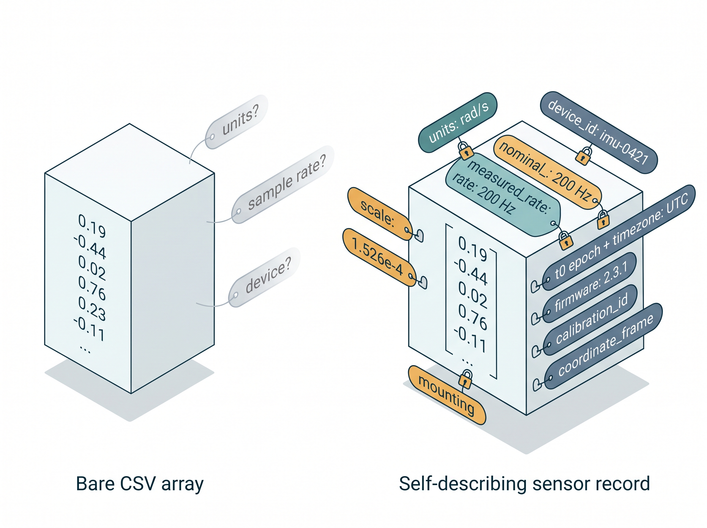
Why it is load-bearing. Consider what breaks without each field. No units, and a fusion stage adds acceleration in \(g\) to acceleration in \(\text{m/s}^2\). No measured rate, and your spectral analysis in Chapter 7 places every peak at the wrong frequency. No calibration version, and a firmware update that changed the gain silently splits your dataset into two incompatible populations. No device ID, and you cannot split train and test by device, arguably the single most important guard against the leakage that Chapter 5 is built around. Metadata is the join key between a raw stream and its physical meaning.

Schemas and standards: agreeing on the record's shape

Why standards exist. Every lab that invents its own metadata layout invents its own way to be incompatible with everyone else, including its future self. Community schemas encode the hard-won list of required fields so you do not rediscover it after losing a dataset. In biosignals, the European Data Format Plus (EDF+) standardized channel labels, per-channel scaling, and annotations for clinical recordings; the neuroimaging world formalized folder-level provenance as the Brain Imaging Data Structure (BIDS). For self-describing arrays, Hierarchical Data Format version 5 (HDF5) and its cloud-native cousin Zarr attach named dimensions and arbitrary attributes directly to the data, so units and sample rate travel inside the file rather than in a fragile sidecar. For sensor descriptions on the web, the World Wide Web Consortium (W3C) SOSA/SSN (Semantic Sensor Network) ontology and Open Geospatial Consortium (OGC) SensorML give a vocabulary for observations, procedures, and platforms. Robotics leans on ROS bag files and message definitions to keep a timestamped, typed record of every topic (as of 2024, ROS 2 and its rosbag2 format have largely replaced the original ROS 1 bags, whose Noetic release reached end-of-life in 2025, though the self-describing, typed-topic discipline is unchanged). What all these standards share, beneath their differing vocabularies, is one organizing principle that a single acronym now names.

The FAIR frame. The unifying principle is that data should be Findable, Accessible, Interoperable, and Reusable (FAIR). In practice FAIR reduces to a discipline you can apply on any project: a stable identifier per recording, a documented schema, units and vocabularies that other tools recognize, and enough provenance that a result can be reproduced. You do not need a heavyweight ontology on day one; you need to pick one self-describing container and never write a bare comma-separated values (CSV) file of unlabeled columns again.

The code below encodes the discipline as a small guard: an ingestion gate that refuses any batch missing the fields required to interpret it, and that flags when the measured rate drifts from the nominal one. Wiring this in front of storage turns a whole class of silent dataset corruption into a loud, early failure.

import numpy as np

REQUIRED = ("device_id", "channel", "units", "scale",
            "nominal_rate_hz", "t0_unix", "timezone",
            "firmware", "calibration_id")

def ingest(samples_raw, timestamps, meta, rate_tol=0.02):
    missing = [k for k in REQUIRED if k not in meta]
    if missing:
        raise ValueError(f"refusing batch: missing metadata {missing}")

    # Verify the delivered rate against the claim; a drift here means
    # dropped samples, a wrong config, or a lying driver.
    dt = np.diff(timestamps)
    measured = 1.0 / np.median(dt)
    if abs(measured - meta["nominal_rate_hz"]) / meta["nominal_rate_hz"] > rate_tol:
        raise ValueError(f"rate mismatch: claimed {meta['nominal_rate_hz']} Hz, "
                         f"measured {measured:.1f} Hz")

    physical = samples_raw.astype(np.float64) * meta["scale"]   # counts -> units
    return {"values": physical, "t": timestamps, "meta": meta,
            "measured_rate_hz": float(measured)}

meta = dict(device_id="imu-0421", channel="gyro_z", units="rad/s", scale=1.526e-4,
            nominal_rate_hz=200.0, t0_unix=1_752_000_000.0, timezone="UTC",
            firmware="2.3.1", calibration_id="cal-2026-05-tumble")
raw = np.random.randint(-2000, 2000, size=1000)
t = meta["t0_unix"] + np.arange(1000) / 200.0
print(ingest(raw, t, meta)["measured_rate_hz"])

import numpy as np, xarray as xr

da = xr.DataArray(
    np.random.randn(1000, 3), dims=("time", "axis"),
    coords={"time": np.arange(1000) / 200.0, "axis": ["x", "y", "z"]},
    attrs={"units": "rad/s", "device_id": "imu-0421",
           "nominal_rate_hz": 200.0, "firmware": "2.3.1"})
da.to_netcdf("gyro.nc")            # units + coords + attrs travel with the data
window = da.sel(time=slice(0.0, 1.0))   # metadata preserved through the slice
print(window.attrs["units"], window.sizes)

What's Next

Chapter 4 leaves the mechanics of getting clean, labeled, timestamped samples behind and turns to what they tell us. The metadata gate here decides whether a number is admissible; the probability toolkit next decides what to believe once it is admitted, giving us estimators, priors, and the aleatoric-versus-epistemic split that lets every later chapter attach honest uncertainty to a sensor reading rather than a bare point estimate.